仮説の定式化と分布

Pythonで学ぶA/Bテスト

Moe Lotfy, PhD

Principal Data Science Manager

仮説の定義

仮説とは:
- 事象を説明する主張
- さらなる検証の出発点
- 検証したいアイデア
強い仮説:
- 検証可能・宣言的・簡潔・論理的
- 体系的な反復を可能にする
- 一般化しやすく理解を確認しやすい
- 実行可能で焦点の定まった提案につながる

仮説の形式

一般的な枠組み:
- Xに基づき、Yを行えば
- Zが起こると考える
- 指標Mで測定する
対立仮説の例:
- ユーザー調査に基づき、チェックアウトページのデザインを更新すれば
- 購入顧客の割合が増える
- 購入率で測定する
帰無仮説: …購入顧客の割合は変わらない…

標本統計量の計算

# Calculate the number of users in groups A and B
n_A = checkout[checkout['checkout_page'] == 'A']['purchased'].count()
n_B = checkout[checkout['checkout_page'] == 'B']['purchased'].count()
print('Group A users:',n_A)
print('Group B users:',n_B)

Group A users: 3000
Group B users: 3000

# Calculate the mean purchase rates of groups A and B
p_A = checkout[checkout['checkout_page'] == 'A']['purchased'].mean()
p_B = checkout[checkout['checkout_page'] == 'B']['purchased'].mean()
print('Group A mean purchase rate:',p_A)
print('Group B mean purchase rate:',p_B)

Group A mean purchase rate: 0.820
Group B mean purchase rate: 0.847

分布のシミュレーションと可視化

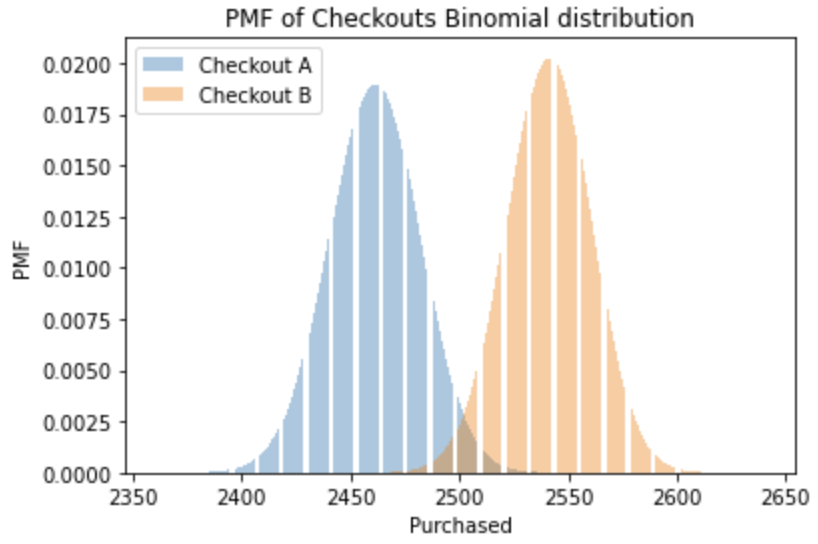
購入確率 p の n 回試行における購入者数は、二項分布に従う。

# Import binom from scipy library 
from scipy.stats import binom 
# Create x-axis range and Binomial distributions A and B
x = np.arange(n_A*p_A - 100, n_B*p_B + 100) 
binom_a = binom.pmf(x, n_A, p_A)
binom_b = binom.pmf(x, n_B, p_B) 
# Plot Binomial distributions A and B
plt.bar(x, binom_a, alpha=0.4, label='Checkout A')
plt.bar(x, binom_b, alpha=0.4, label='Checkout B')
plt.xlabel('Purchased')
plt.ylabel('PMF')
plt.title('PMF of Checkouts Binomial distribution')
plt.show()

チェックアウトA・Bグループの二項分布

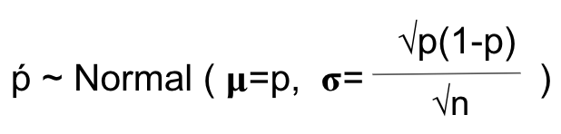
中心極限定理

十分大きい標本サイズでは、標本平均 p の分布は

真の母平均のまわりで正規分布する
標準偏差 = 平均の標準誤差
元のデータ分布に依存しない

比率における中心極限定理の式

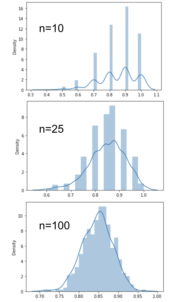
Pythonでの中心極限定理

# Set random seed for repeatability 
np.random.seed(47)
# Create an empty list to hold means
sampled_means = []
# Create loop to simulate 1000 sample means
for i in range(1000):
    # Take a sample of n=100
    sample = checkout['purchased'].sample(100,replace=True)
    # Get the sample mean and append to list
    sample_mean = np.mean(sample)
    sampled_means.append(sample_mean)
# Plot distribution
sns.displot(sampled_means, kde=True)
plt.show()

中心極限定理のPythonデモ。標本サイズが大きいほど分布は正規に近づく

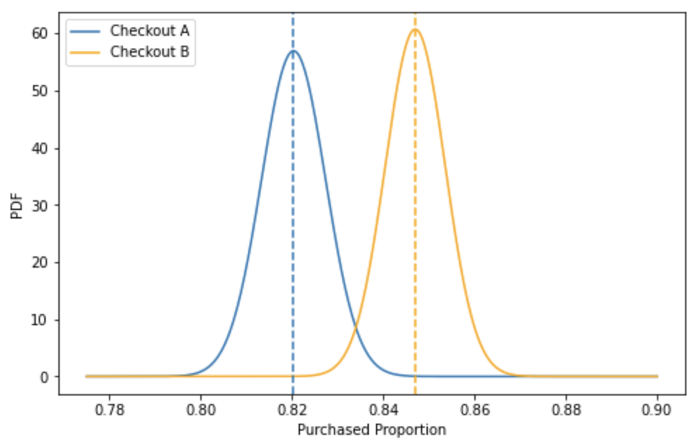
仮説の数理表現

# Import norm from scipy library 
from scipy.stats import norm
# Create x-axis range and normal distributions A and B
x = np.linspace(0.775, 0.9, 500)
norm_a = norm.pdf(x, p_A, np.sqrt(p_A*(1-p_A) / n_A))
norm_b = norm.pdf(x, p_B, np.sqrt(p_B*(1-p_B) / n_B))
# Plot normal distributions A and B
sns.lineplot(x=x, y=norm_a, ax=ax, label='Checkout A')
sns.lineplot(x=x, y=norm_b, color='orange', \
             ax=ax, label= 'Checkout B')
ax.axvline(p_A, linestyle='--')
ax.axvline(p_B, linestyle='--')
plt.xlabel('Purchased Proportion')
plt.ylabel('PDF')
plt.legend(loc="upper left")
plt.show()

帰無仮説と対立仮説の平均差プロット

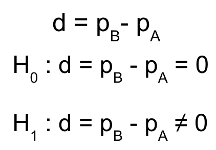
帰無仮説と対立仮説の数式表現

練習に進みましょう！

Pythonで学ぶA/Bテスト