時系列を定常化する

Pythonで学ぶARIMAモデル

James Fulton

Climate informatics researcher

概要

定常性の統計的検定
データを定常化する方法

拡張Dickey–Fuller検定

トレンド非定常性の検定
帰無仮説: 時系列は非定常

adfuller検定の実行

from statsmodels.tsa.stattools import adfuller

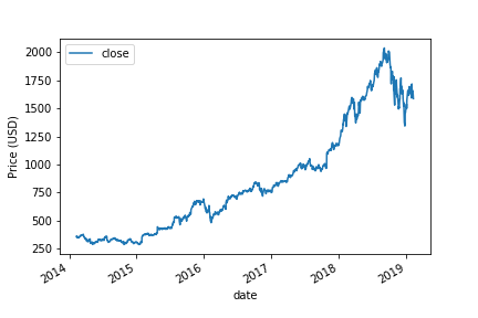
results = adfuller(df['close'])

結果の解釈

print(results)

(-1.34, 0.60, 23, 1235, {'1%': -3.435, '5%': -2.913, '10%': -2.568}, 10782.87)

0番目は検定統計量 (-1.34)
- 値が小さい（より負）ほど定常である可能性が高い

1番目はp値 (0.60)
- p値が小さければ帰無仮説を棄却 → 非定常を棄却

4番目は臨界値

結果の解釈

print(results)

(-1.34, 0.60, 23, 1235, {'1%': -3.435, '5%': -2.863, '10%': -2.568}, 10782.87)

0番目は検定統計量 (-1.34)
- 値が小さい（より負）ほど定常である可能性が高い

1番目はp値 (0.60)
- p値が小さければ帰無仮説を棄却 → 非定常を棄却

4番目は臨界値

¹ https://www.statsmodels.org/dev/generated/statsmodels.tsa.stattools.adfuller.html

プロットの価値

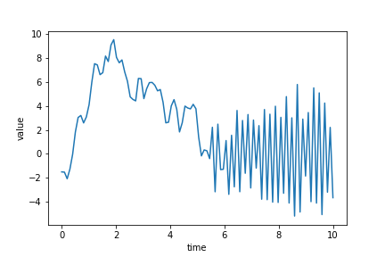
可視化は誤った仮定を防ぐ

プロットの価値

時系列を定常化する方法

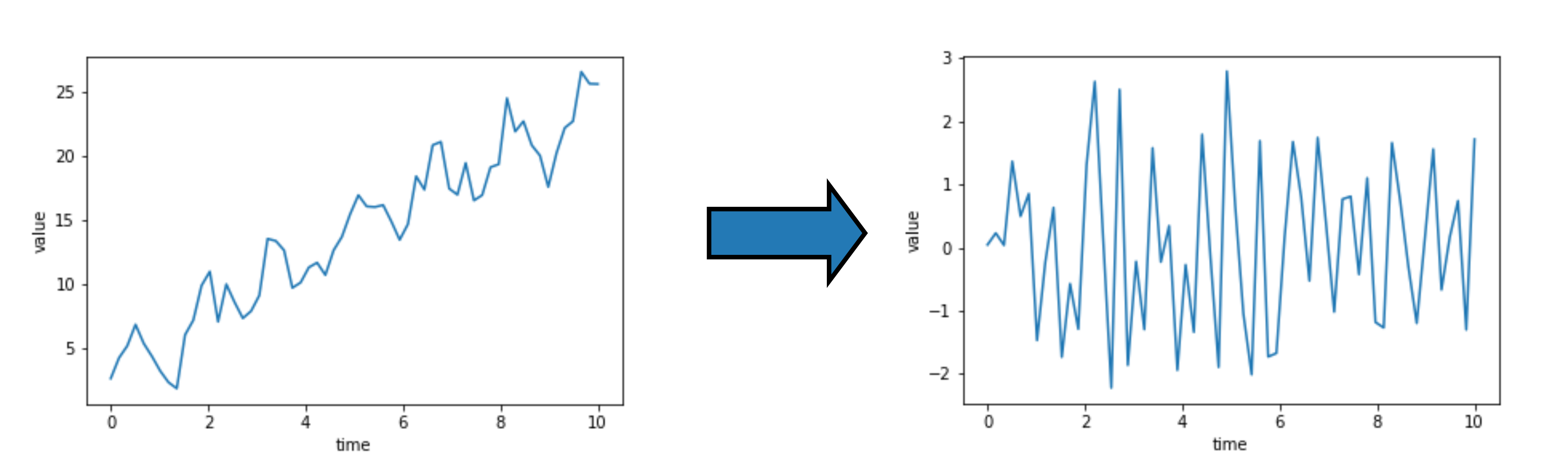
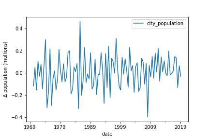
差分をとる

差分: $\Delta y_t = y_t - y_{t-1}$

差分をとる

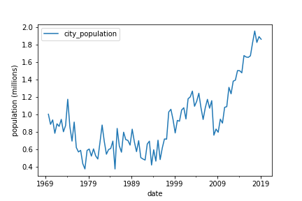
df_stationary = df.diff()

            city_population
date                       
1969-09-30              NaN
1970-03-31        -0.116156
1970-09-30         0.050850
1971-03-31        -0.153261
1971-09-30         0.108389

差分をとる

df_stationary = df.diff().dropna()

            city_population
date                       
1970-03-31        -0.116156
1970-09-30         0.050850
1971-03-31        -0.153261
1971-09-30         0.108389
1972-03-31        -0.029569

差分をとる

その他の変換

他の変換の例

対数をとる
- np.log(df)
平方根をとる
- np.sqrt(df)
変化率をとる
- df.shift(1)/df

Let's practice!

Pythonで学ぶARIMAモデル