ビニングと特徴エンジニアリング

Machine Learning with PySpark

Andrew Collier

Data Scientist, Fathom Data

ビニング

連続値をビンにグループ化

身長のビニング

身長のヒストグラム

+------+
|height|
+------+
|  1.42|
|  1.45|
|  1.47|
|  1.50|
|  1.52|
|  1.57|
|  1.60|
|  1.75|
|  1.85|
|  1.88|
+------+

身長のビニング

範囲付きの身長ヒストグラム

+------+
|height|
+------+
|  1.42|
|  1.45|
|  1.47|
|  1.50|
|  1.52|
|  1.57|
|  1.60|
|  1.75|
|  1.85|
|  1.88|
+------+

身長のビニング

範囲とラベル付きの身長ヒストグラム

+------+
|height|
+------+
|  1.42|
|  1.45|
|  1.47|
|  1.50|
|  1.52|
|  1.57|
|  1.60|
|  1.75|
|  1.85|
|  1.88|
+------+

身長のビニング

範囲とラベル付きの身長ヒストグラム

+------+----------+
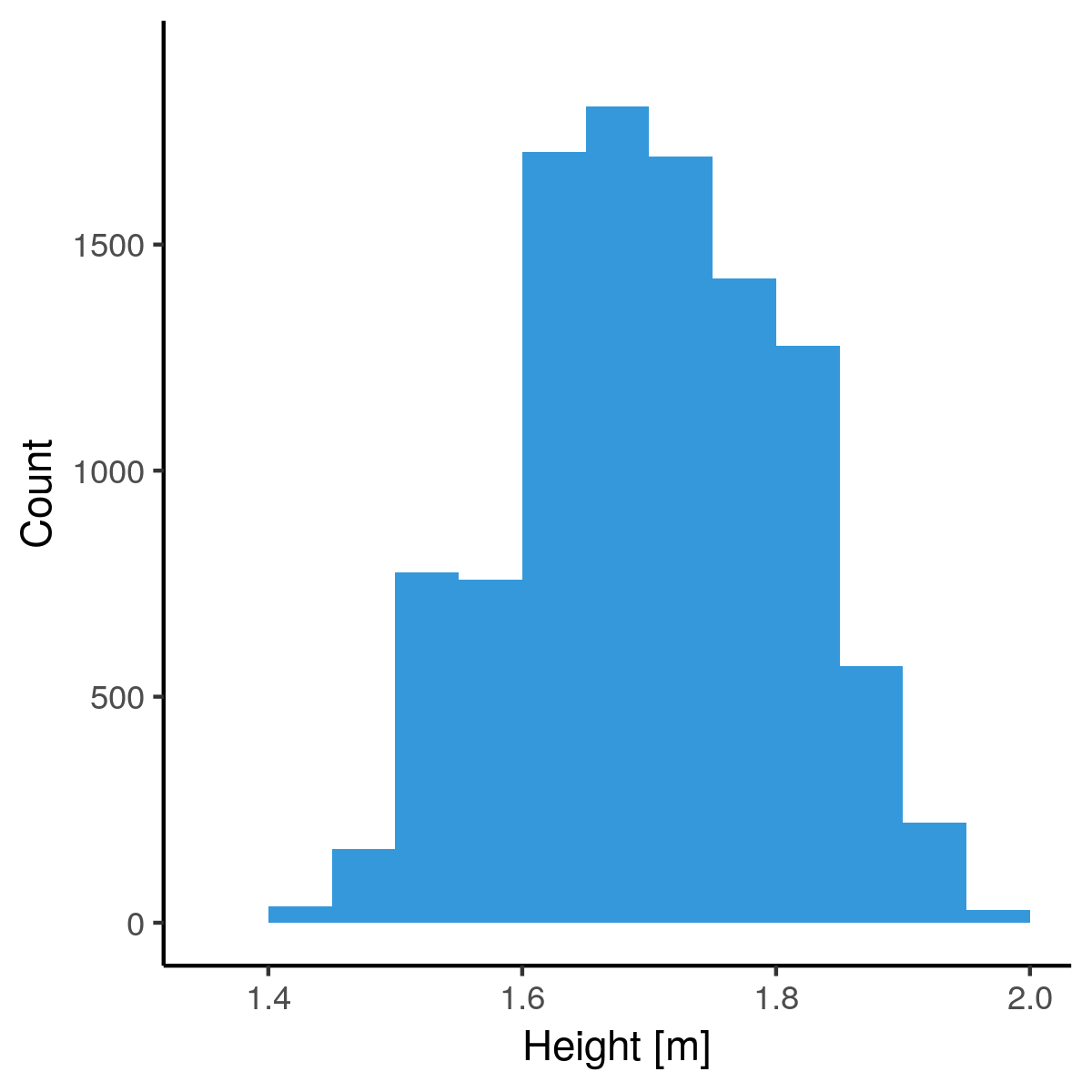
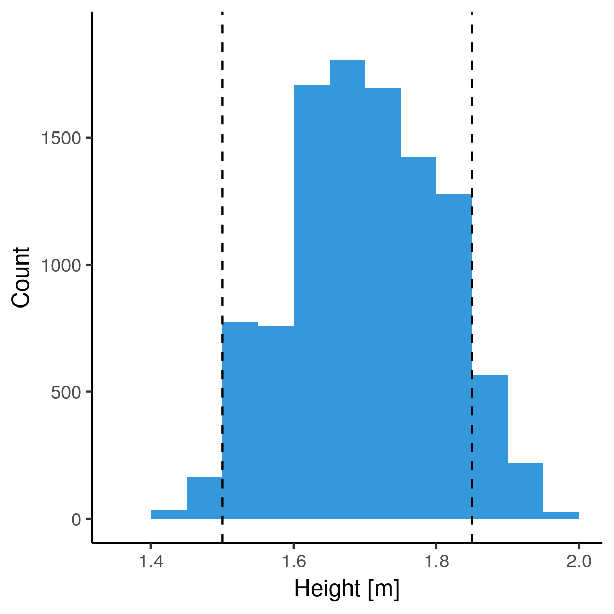
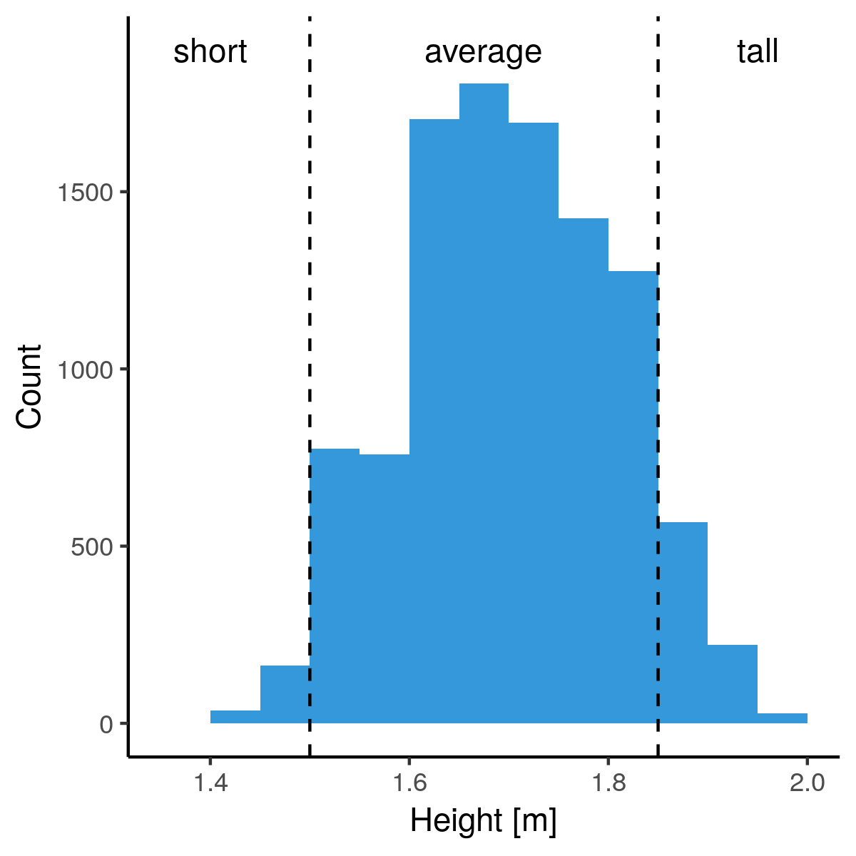
|height|height_bin|
+------+----------+
|  1.42|     short|
|  1.45|     short|
|  1.47|     short|
|  1.50|     short|
|  1.52|   average|
|  1.57|   average|
|  1.60|   average|
|  1.75|   average|
|  1.85|      tall|
|  1.88|      tall|
+------+----------+

RPMのヒストグラム

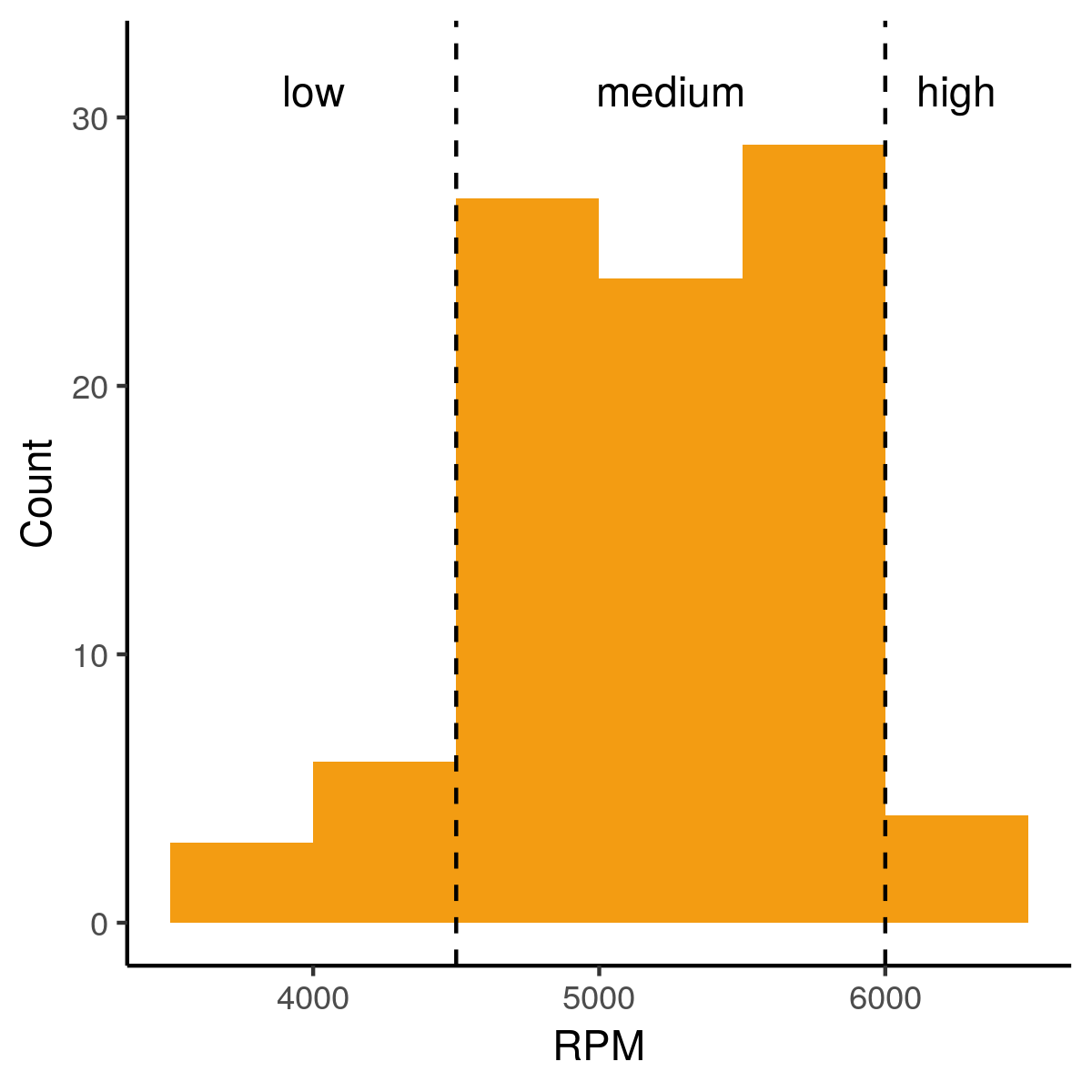
車のRPMには「自然な」区切りがあります:

$\text{RPM} < 4500$ — low
$\text{RPM} > 6000$ — high
それ以外 — medium

範囲とラベル付きのRPMヒストグラム

RPMのビン

from pyspark.ml.feature import Bucketizer

bucketizer = Bucketizer(splits=[3500, 4500, 6000, 6500],
                        inputCol="rpm",
                        outputCol="rpm_bin")

rpm列にビンを適用します。

bucketed = bucketizer.transform(cars)

RPMのビン

bucketed.select('rpm', 'rpm_bin').show(5)

+----+-------+
| rpm|rpm_bin|
+----+-------+
|3800|    0.0|
|4500|    1.0|
|5750|    1.0|
|5300|    1.0|
|6200|    2.0|
+----+-------+

bucketed.groupBy('rpm_bin').count().show()

+-------+-----+
|rpm_bin|count|
+-------+-----+
|    0.0|    8| <- low
|    1.0|   67| <- medium
|    2.0|   17| <- high
+-------+-----+

RPMビンのワンホット化

RPMのビンをワンホットでダミー変数化します。

+-------+-------------+
|rpm_bin|    rpm_dummy|
+-------+-------------+
|    0.0|(2,[0],[1.0])| <- low
|    1.0|(2,[1],[1.0])| <- medium
|    2.0|    (2,[],[])| <- high
+-------+-------------+

'high'のRPMビンは基準水準のためダミーは作成されません。

ビン化したRPMでのモデル

regression.coefficients

DenseVector([1.3814, 0.1433])

+-------+-------------+
|rpm_bin|    rpm_dummy|
+-------+-------------+
|    0.0|(2,[0],[1.0])| <- low
|    1.0|(2,[1],[1.0])| <- medium
|    2.0|    (2,[],[])| <- high
+-------+-------------+

regression.intercept

8.1835

'low' RPMの消費量:

8.1835 + 1.3814 = 9.5649

'medium' RPMの消費量:

8.1835 + 0.1433 = 8.3268

追加の特徴エンジニアリング

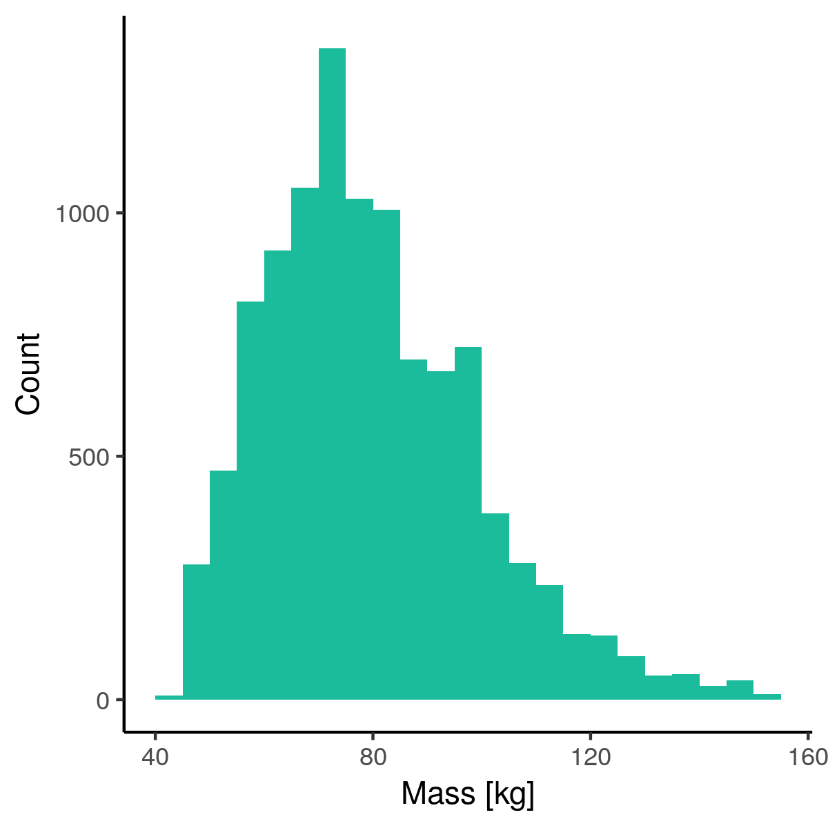
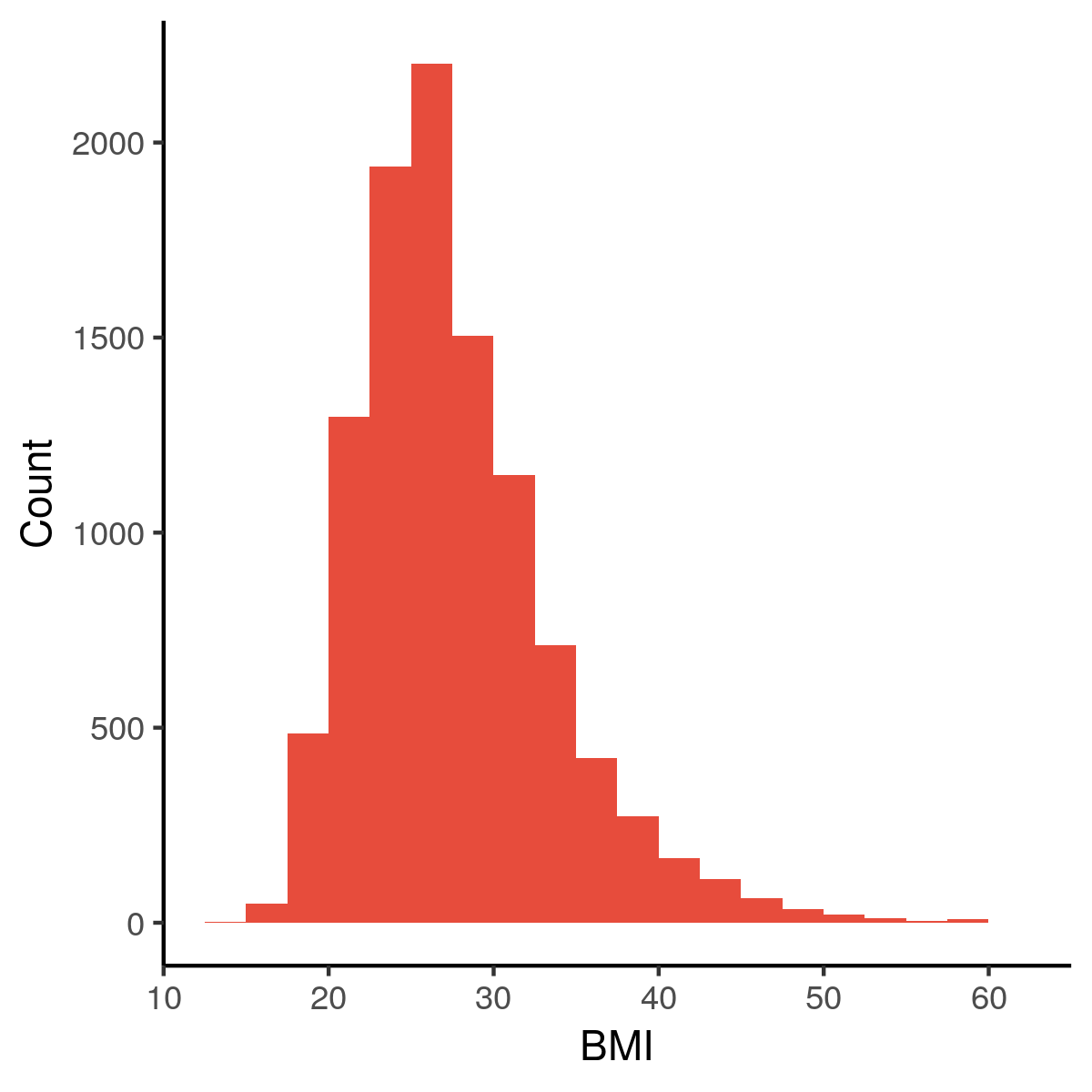
単一列への演算:

log()
sqrt()
pow()

2列間の演算:

質量・身長からBMIへ

身長のヒストグラム

体重のヒストグラム

質量・身長からBMIへ

BMIのヒストグラム

+------+-----+----+
|height| mass| bmi|    bmi = mass / height^2
+------+-----+----+
|  1.52| 77.1|33.2|
|  1.60| 58.1|22.7|
|  1.57|122.0|49.4|
|  1.75| 95.3|31.0|
|  1.80| 99.8|30.7|
|  1.65| 90.7|33.3|
|  1.60| 70.3|27.5|
|  1.78| 81.6|25.8|
|  1.65| 77.1|28.3|
|  1.78|128.0|40.5|
+------+-----+----+

密度のエンジニアリング

cars = cars.withColumn('density_line', cars.mass / cars.length)       # Linear density
cars = cars.withColumn('density_quad', cars.mass / cars.length**2)    # Area density
cars = cars.withColumn('density_cube', cars.mass / cars.length**3)    # Volume density

+------+------+------------+------------+------------+
|  mass|length|density_line|density_quad|density_cube|
+------+------+------------+------------+------------+
|1451.0| 4.775|303.87434554|63.638606397|13.327456837|
|1129.0| 4.623|244.21371403|52.825808790|11.426737787|
|1399.0| 4.547|307.67539036|67.665579583|14.881367843|
+------+------+------------+------------+------------+

特徴を作ってみましょう！

Machine Learning with PySpark