R での tidymodels によるモデリング
David Svancer
Data Scientist
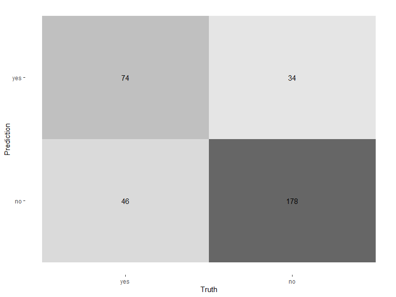
autoplot() でヒートマップ
autoplot() に渡すtype を 'heatmap' に設定
conf_mat(leads_results, truth = purchased, estimate = .pred_class) %>%autoplot(type = 'heatmap')

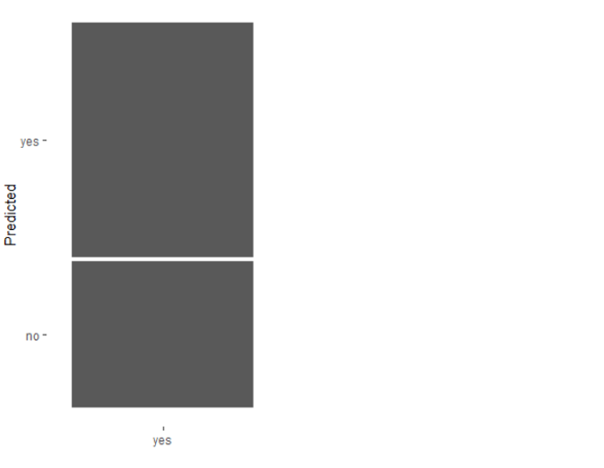
autoplot() でモザイク
type を 'mosaic' に設定
conf_mat(leads_results,
truth = purchased,
estimate = .pred_class) %>%
autoplot(type = 'mosaic')

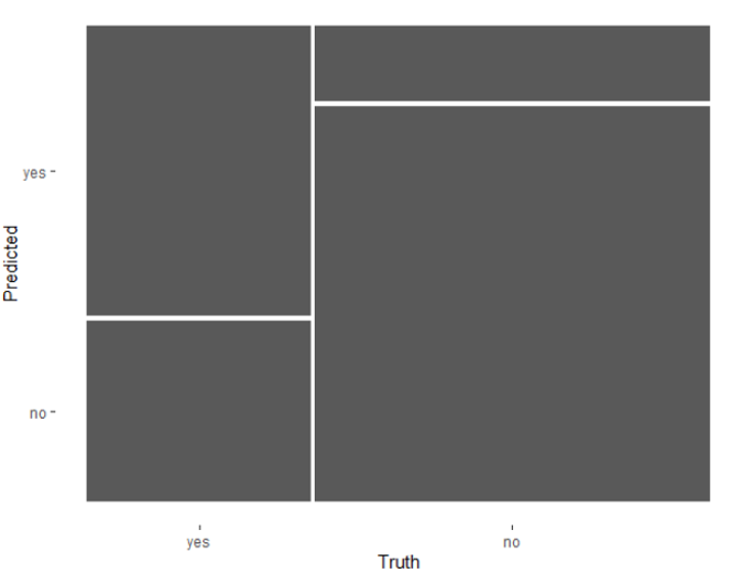
autoplot() でモザイク
type を 'mosaic' に設定conf_mat(leads_results,
truth = purchased,
estimate = .pred_class) %>%
autoplot(type = 'mosaic')

二値分類の既定しきい値は 0.5
leads_results
.pred_yes が 0.5 以上なら、tidymodels の predict() により .pred_class は 'yes' になりますleads_results
# A tibble: 332 x 4
purchased .pred_class .pred_yes .pred_no
<fct> <fct> <dbl> <dbl>
1 no no 0.134 0.866
2 yes yes 0.729 0.271
3 no no 0.133 0.867
4 no no 0.0916 0.908
5 yes yes 0.598 0.402
6 no no 0.128 0.872
7 yes no 0.112 0.888
8 no no 0.169 0.831
9 no no 0.158 0.842
10 yes yes 0.520 0.480
# ... with 322 more rows
しきい値を変えると分類モデルの性能はどう変わるか?
.pred_yes 列にある一意のしきい値
| しきい値 | 特異度 | 感度 |
|---|---|---|
| 0 | 0 | 1 |
| 0.11 | 0.01 | 0.98 |
| 0.15 | 0.05 | 0.97 |
| ... | ... | ... |
| 0.84 | 0.89 | 0.08 |
| 0.87 | 0.94 | 0.02 |
| 0.91 | 0.99 | 0 |
| 1 | 1 | 0 |
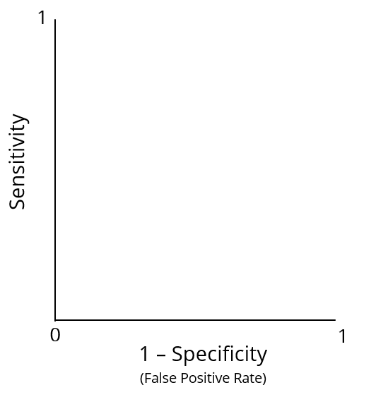
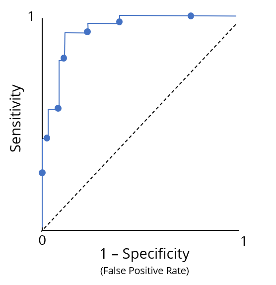
ROC(受信者動作特性)曲線
ROC(受信者動作特性)曲線

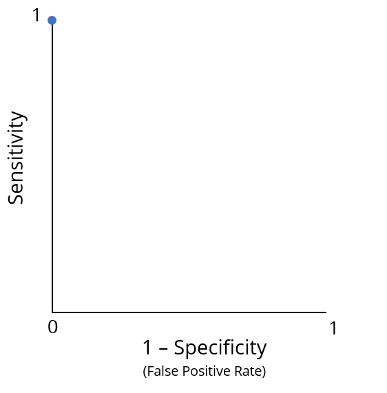
最適性能は点 (0, 1)
最適性能は点 (0, 1)
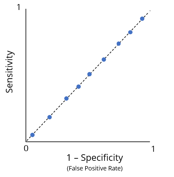
低性能

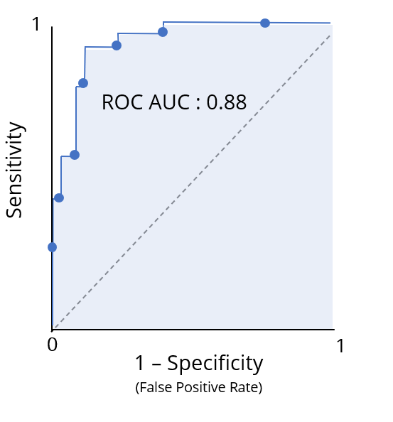
ROC 曲線下面積(ROC AUC)は、分類モデルの ROC 情報を1つの数値に要約します
成績評価風の目安

roc_curve() 関数
truth 列leads_results では .pred_yes
.pred_yes の一意のしきい値すべてに対する特異度と感度の tibble を返しますleads_results %>%
roc_curve(truth = purchased, .pred_yes)
# A tibble: 331 x 3
.threshold specificity sensitivity
<dbl> <dbl> <dbl>
1 -Inf 0 1
2 0.0871 0 1
3 0.0888 0.00472 1
4 0.0893 0.00943 1
5 0.0896 0.0142 1
6 0.0902 0.0142 0.992
7 0.0916 0.0142 0.983
8 0.0944 0.0189 0.983
# ... with 323 more rows
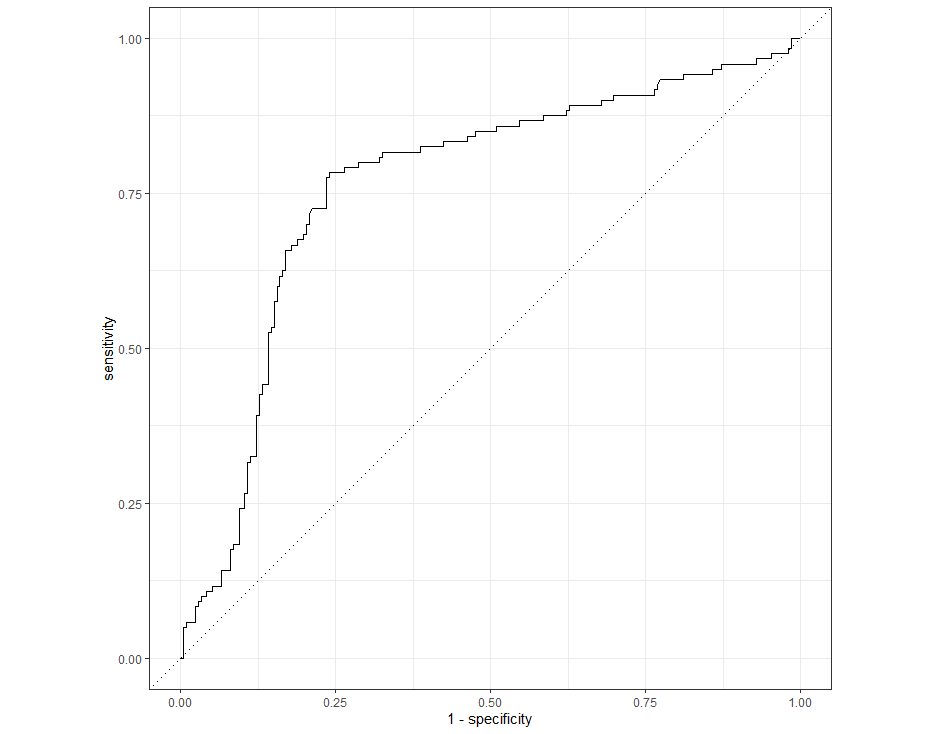
roc_curve() の結果を autoplot() に渡すと、ROC 曲線が描画されます
leads_results %>%
roc_curve(truth = purchased, .pred_yes) %>%
autoplot()

yardstick の roc_auc() 関数は ROC AUC を計算します
truth 列roc_auc(leads_results,
truth = purchased,
.pred_yes)
# A tibble: 1 x 3
.metric .estimator .estimate
<chr> <chr> <dbl>
1 roc_auc binary 0.763
R での tidymodels によるモデリング