セグメントを把握・解釈する

Pythonで学ぶカスタマーセグメンテーション

Karolis Urbonas

Head of Data Science, Amazon

顧客ペルソナの作り方

各クラスタの要約統計（例：平均RFM）
スネークプロット（市場調査由来）
母集団と比べたクラスタ属性の相対的重要度

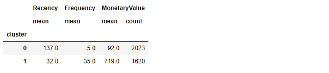
各クラスタの要約統計

推奨値の前後で複数の k を使ってk-meansを実行

元のDataFrameにクラスタラベル列を作成：

datamart_rfm_k2 = datamart_rfm.assign(Cluster = cluster_labels)

各クラスタの平均RFMとサイズを計算：

datamart_rfm_k2.groupby(['Cluster']).agg({
   'Recency': 'mean',
   'Frequency': 'mean',
   'MonetaryValue': ['mean', 'count'],
}).round(0)

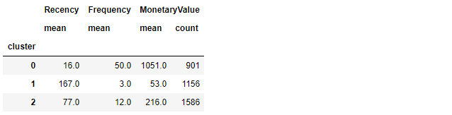
k=3 でも同様に実施

各クラスタの要約統計

各クラスタリング解の平均RFMを比較

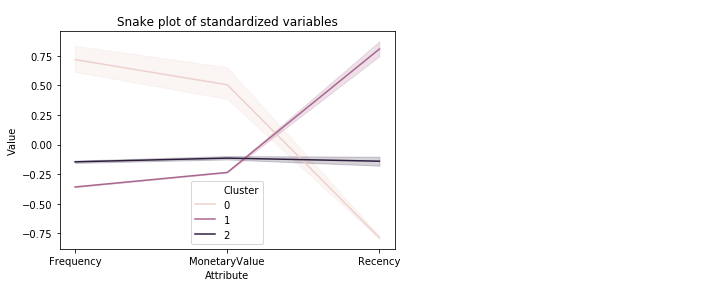
スネークプロットでセグメントを理解・比較

セグメント比較の市場調査手法
各セグメントの属性を可視化
まず正規化（中心化・標準化）が必要
各属性のクラスタ平均（正規化済み）をプロット

スネークプロット用のデータ準備

datamart_normalized をDataFrame化し、Cluster 列を追加

datamart_normalized = pd.DataFrame(datamart_normalized, 
                                   index=datamart_rfm.index, 
                                   columns=datamart_rfm.columns)
datamart_normalized['Cluster'] = datamart_rfm_k3['Cluster']

データをロング形式へ。RFM値と指標名を各1列に格納

datamart_melt = pd.melt(datamart_normalized.reset_index(), 
                    id_vars=['CustomerID', 'Cluster'],
                    value_vars=['Recency', 'Frequency', 'MonetaryValue'], 
                    var_name='Attribute', 
                    value_name='Value')

スネークプロットを可視化する

plt.title('Snake plot of standardized variables')
sns.lineplot(x="Attribute", y="Value", hue='Cluster', data=datamart_melt)

セグメント属性の相対的重要度

各セグメント属性の相対的重要度を把握する有用な手法
各クラスタの平均を計算
母集団の平均を計算
重要度 = クラスタ平均 ÷ 母集団平均 − 1（同値なら0）

cluster_avg = datamart_rfm_k3.groupby(['Cluster']).mean()

population_avg = datamart_rfm.mean()

relative_imp = cluster_avg / population_avg - 1

相対的重要度を分析・プロット

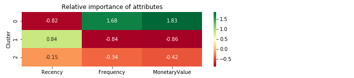
比率が0から離れるほど、その属性の重要度（母集団比）は高い

relative_imp.round(2)

         Recency  Frequency  MonetaryValue
Cluster                                   
0          -0.82       1.68           1.83
1           0.84      -0.84          -0.86
2          -0.15      -0.34          -0.42

# Plot heatmap
plt.figure(figsize=(8, 2))
plt.title('Relative importance of attributes')
sns.heatmap(data=relative_imp, annot=True, fmt='.2f', cmap='RdYlGn')
plt.show()

相対的重要度のヒートマップ

         Recency  Frequency  MonetaryValue
Cluster                                   
0          -0.82       1.68           1.83
1           0.84      -0.84          -0.86
2          -0.15      -0.34          -0.42

さまざまな顧客プロファイリング手法を試しましょう！

Pythonで学ぶカスタマーセグメンテーション