コロプレスマップ

R で学ぶ plotly によるインタラクティブ可視化

Adam Loy

Statistician, Carleton College

世界の人口密度マップ（800px）

plotlyでのコロプレスマップ

head(turnout)

       state state.abbr turnout2018 turnout2014  ballots      vep      vap
1    Alabama         AL       0.474       0.332  1725000  3641209  3802714
2     Alaska         AK       0.537       0.548   280000   521777   554426
3    Arizona         AZ       0.486       0.341  2385000  4910625  5519036
4   Arkansas         AR       0.412       0.403   895000  2171940  2319740
5 California         CA       0.478       0.307 12250000 25635139 30836229
6   Colorado         CO       0.619       0.547  2540000  4103903  4445013

plotlyでのコロプレスマップ

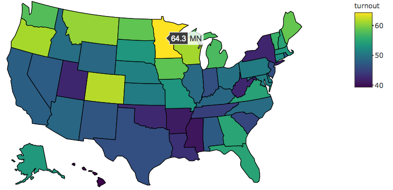
turnout %>%

  plot_geo(locationmode = 'USA-states') %>%

  add_trace(
    z = ~turnout,                   # 色の値を設定
    locations = ~state.abbr         # 事例をポリゴンに対応付け
  ) %>%

  layout(geo = list(scope = 'usa')) # 米国のみを表示

plot_geo() の制約

locationmode: "USA-states" | "ISO-3" | "country names"

マッピングのオプション

scope = "usa"

"world" | "usa" | "europe" | "asia" | "africa" | "north america" | "south america"

projection = list(type = "mercator")

"conic conformal" | "mercator" | "robinson" | "stereographic" | ほか18種類

scale = 1

大きい値ほどズームイン

center = list(lat = ~c.lat, lon = ~c.lon)

地図の中心を c.lat と c.lon で指定

さあ、地図を作りましょう！

R で学ぶ plotly によるインタラクティブ可視化