モデルの誤差とランダム性

Pythonで学ぶ線形モデリング入門

Jason Vestuto

Data Scientist

誤差の種類

  1. 測定誤差
    • 例:センサーの故障、測定値の誤記録
  2. サンプリングバイアス
    • 例:気温データが最も暑い8月のみ
  3. 偶然性
Pythonで学ぶ線形モデリング入門

帰無仮説

問い:この効果は関係性によるものか、偶然によるものか?

答え:帰無仮説を確認する。

Pythonで学ぶ線形モデリング入門

整列データ

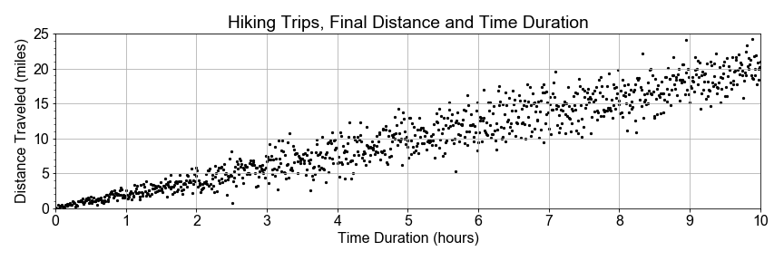
ハイキングデータの散布図。横軸は所要時間(時間)、縦軸は移動距離(マイル)

Pythonで学ぶ線形モデリング入門

データのグループ化

ハイキングデータの散布図。横軸は所要時間(時間)、縦軸は移動距離(マイル)。5時間未満を赤、5時間以上を青で表示

Pythonで学ぶ線形モデリング入門

データのグループ化

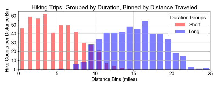
2つのヒストグラム。赤(短時間グループ)は約5マイル中心、青(長時間グループ)は約15マイル中心の釣り鐘型

  • 短時間グループ、平均 = 5
  • 長時間グループ、平均 = 15
Pythonで学ぶ線形モデリング入門

検定統計量

# Group into early and late times
group_short = sample_distances[times < 5]
group_long = sample_distances[times > 5]
# Resample distributions
resample_short = np.random.choice(group_short, size=500, replace=True)
resample_long = np.random.choice(group_long, size=500, replace=True)
# Test Statistic
test_statistic = resample_long - resample_short
# Effect size as mean of test statistic distribution
effect_size = np.mean(test_statistic)
Pythonで学ぶ線形モデリング入門

シャッフルと再グループ化

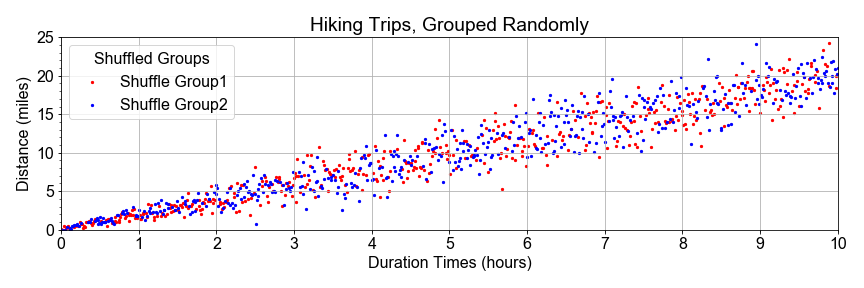
ハイキングデータの散布図。横軸は所要時間(時間)、縦軸は移動距離(マイル)。すべての時間帯にわたって赤と青のデータが混在している

Pythonで学ぶ線形モデリング入門

シャッフルと再グループ化

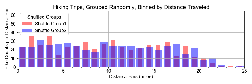
ほぼ完全に重なり合う2つのヒストグラム。0〜25マイルの範囲で、ほぼ同じ形状

Pythonで学ぶ線形モデリング入門

シャッフルと分割

# Concatenate and Shuffle
shuffle_bucket = np.concatenate((group_short, group_long))
np.random.shuffle(shuffle_bucket)
# Split in the middle
slice_index = len(shuffle_bucket)//2
shuffled_half1 = shuffle_bucket[0:slice_index]
shuffled_half2 = shuffle_bucket[slice_index+1:]
Pythonで学ぶ線形モデリング入門

再サンプリングと再検定

# Resample shuffled populations
shuffled_sample1 = np.random.choice(shuffled_half1, size=500, replace=True)
shuffled_sample2 = np.random.choice(shuffled_half2, size=500, replace=True)
# Recompute effect size
shuffled_test_statistic = shuffled_sample2 - shuffled_sample1
effect_size = np.mean(shuffled_test_statistic)
Pythonで学ぶ線形モデリング入門

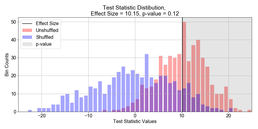
p値

横軸に検定統計量、縦軸にビン数をとった2つのヒストグラム。青はx=0付近に広く分布し、赤はx=10付近に狭く分布。x=10に垂直な黒線

Pythonで学ぶ線形モデリング入門

練習しましょう!

Pythonで学ぶ線形モデリング入門

Preparing Video For Download...