予測モデリングの背景

tidyverse で学ぶモデリング

Albert Y. Kim

Assistant Professor of Statistical and Data Sciences

予測モデリングの例

ワシントン州キング郡（シアトル近郊）の住宅価格データセット（Kaggle.com で公開）。

問い: 住宅の特徴から販売価格を予測できるか？

変数:

$y$: 住宅販売 price（米ドル）
$\vec{x}$: sqft_living、condition、bedrooms、yr_built、waterfront などの特徴量

予測モデリングの例

moderndive パッケージ（ModernDive）より：

library(dplyr)
library(moderndive)
glimpse(house_prices)

Observations: 21,613
Variables: 21
$ id            <chr> "7129300520", "6414100192"...
$ date          <dttm> 2014-10-13, 2014-12-09, 2015...
$ price         <dbl> 221900, 538000, 180000, 604000...
...

探索的データ分析

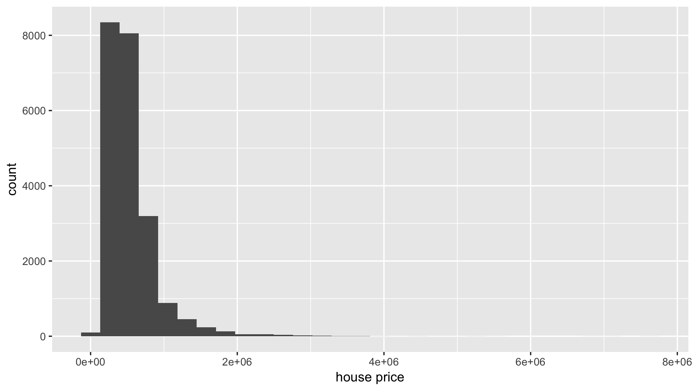
library(ggplot2)
ggplot(house_prices, aes(x = price)) +
  geom_histogram() + 
  labs(x = "house price", y = "count")

目的変数のヒストグラム

Gapminderデータ

x軸のLog10スケーリング

Log10変換

# log10() transform price and size
house_prices <- house_prices %>%
  mutate(log10_price = log10(price)) %>% 
  select(price, log10_price)

# A tibble: 21,613 x 2
     price log10_price
     <dbl>       <dbl>
 1  221900        5.35
 2  538000        5.73
 3  180000        5.26
 4  604000        5.78
 5  510000        5.71
 6 1225000        6.09

新しい目的変数のヒストグラム

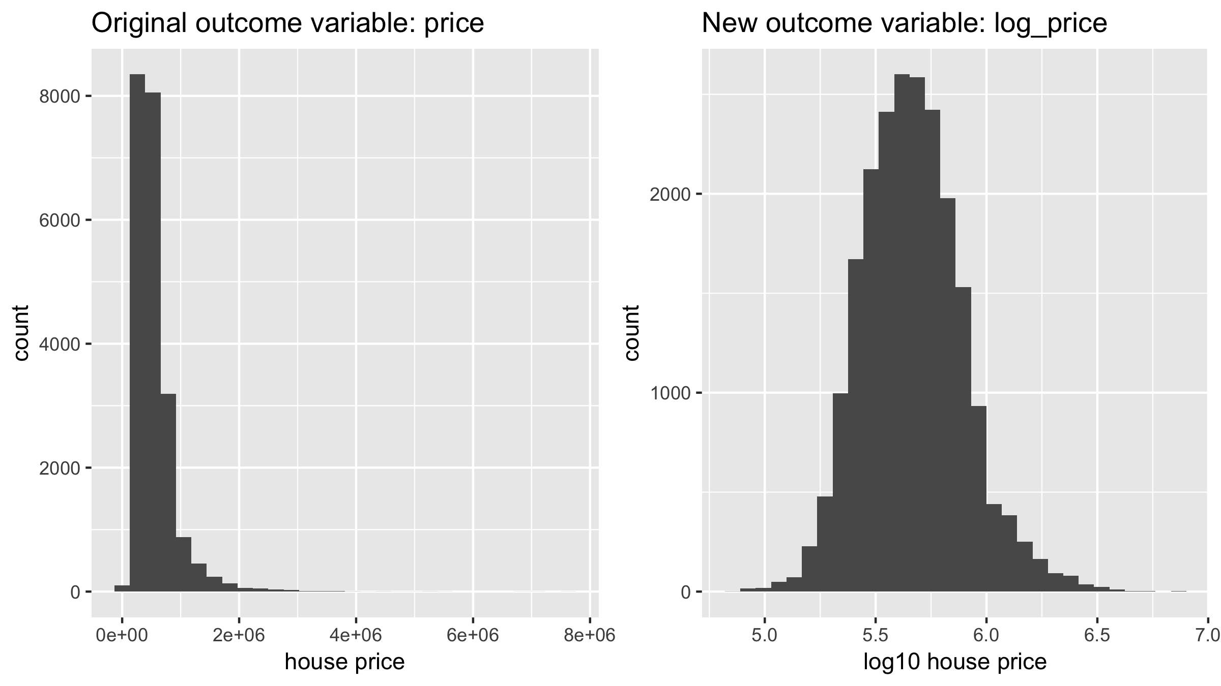
# Histogram of original outcome variable
ggplot(house_prices, aes(x = price)) +
  geom_histogram() + 
  labs(x = "house price", y = "count")

# Histogram of new, log10-transformed outcome variable
ggplot(house_prices, aes(x = log10_price)) +
  geom_histogram() + 
  labs(x = "log10 house price", y = "count")

Log10変換の前後比較

練習しましょう！

tidyverse で学ぶモデリング