tidyverse で学ぶモデリング
Albert Y. Kim
Assistant Professor of Statistical and Data Sciences
$y = f(\vec{x}) + \epsilon$ を考えます。
モデリング目的の主な違い:
house_prices %>%
  select(log10_price, condition) %>%
  glimpse()
Observations: 21,613
Variables: 2
$ log10_price <dbl> 5.346157, 5.730782, 5.255273...
$ condition   <fct> 3, 3, 3, 5, 3, 3, 3, 3, 3, 3, 3...
library(ggplot2)
library(dplyr)
library(moderndive)

# Apply log10-transformation to outcome variable
house_prices <- house_prices %>%
  mutate(log10_price = log10(price))

# Boxplot
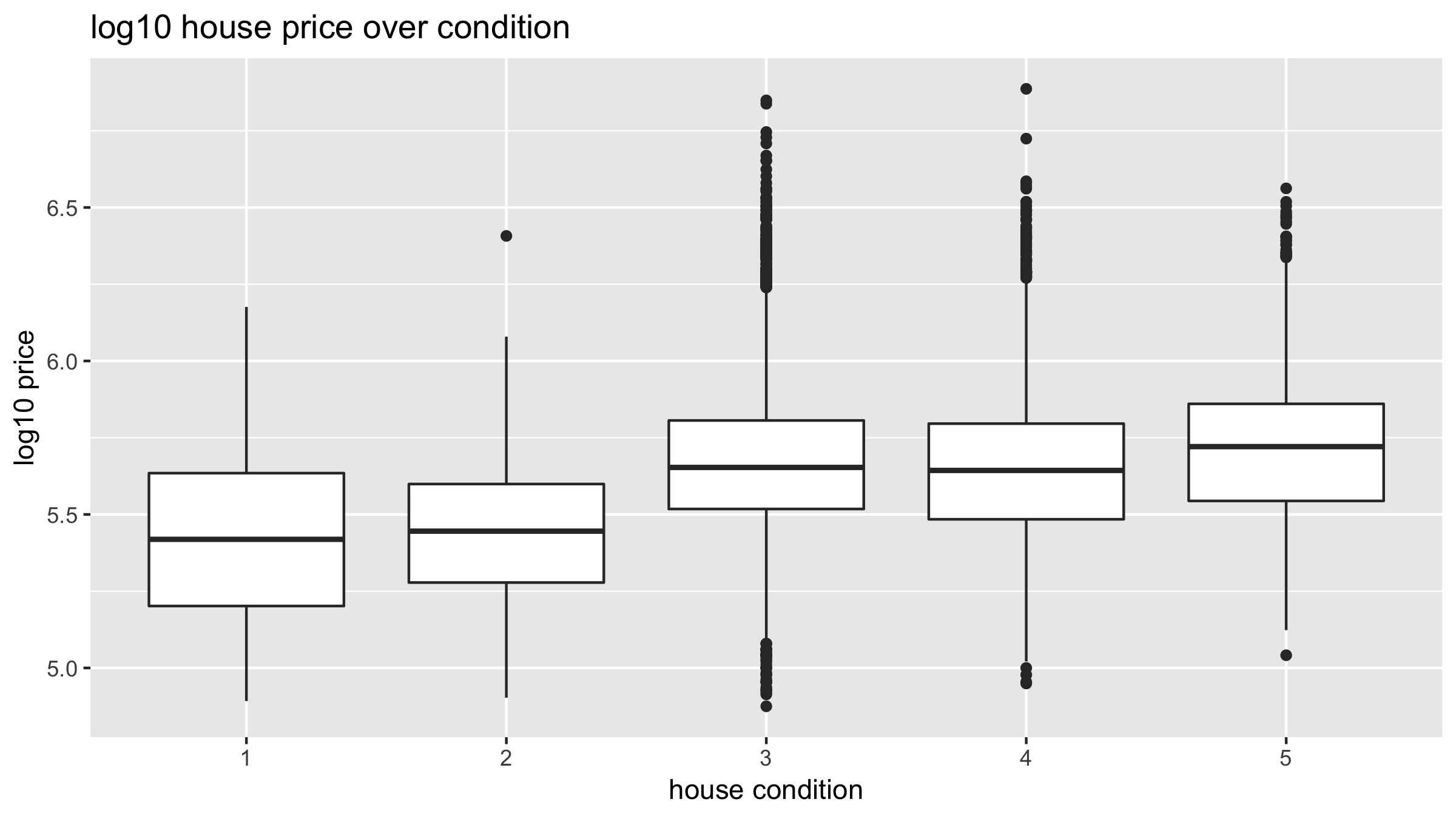
ggplot(house_prices, aes(x = condition, y = log10_price)) +
  geom_boxplot() +
  labs(x = "house condition", y = "log10 price",
       title = "log10 house price over condition")
library(ggplot2) library(dplyr) library(moderndive) # Apply log10-transformation to outcome variable house_prices <- house_prices %>% mutate(log10_price = log10(price))
# Boxplot ggplot(house_prices, aes(x = condition, y = log10_price)) + geom_boxplot() + labs(x = "house condition", y = "log10 price", title = "log10 house price over condition")
house_prices %>%
  group_by(condition) %>%
  summarize(mean = mean(log10_price),
            sd = sd(log10_price), n = n())
# A tibble: 5 x 4
  condition  mean    sd     n
  <fct>     <dbl> <dbl> <int>
1 1          5.42 0.293    30
2 2          5.45 0.233   172
3 3          5.67 0.224 14031
4 4          5.65 0.228  5679
5 5          5.71 0.244  1701
# Prediction for new house with condition 4 in dollars
10^(5.65)
446683.6