動的調和回帰
Rで学ぶ予測入門

Rob J. Hyndman
Professor of Statistics at Monash University
動的調和回帰

動的調和回帰
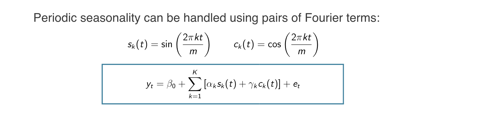
$m =$ 季節周期
任意の周期関数は、十分大きいKで sin・cos の和で近似可能
回帰係数: $\alpha_k$, $\gamma_k$
$e_t$ は非季節 ARIMA でモデル化可
季節パターンは不変と仮定
例: オーストラリアのカフェ支出
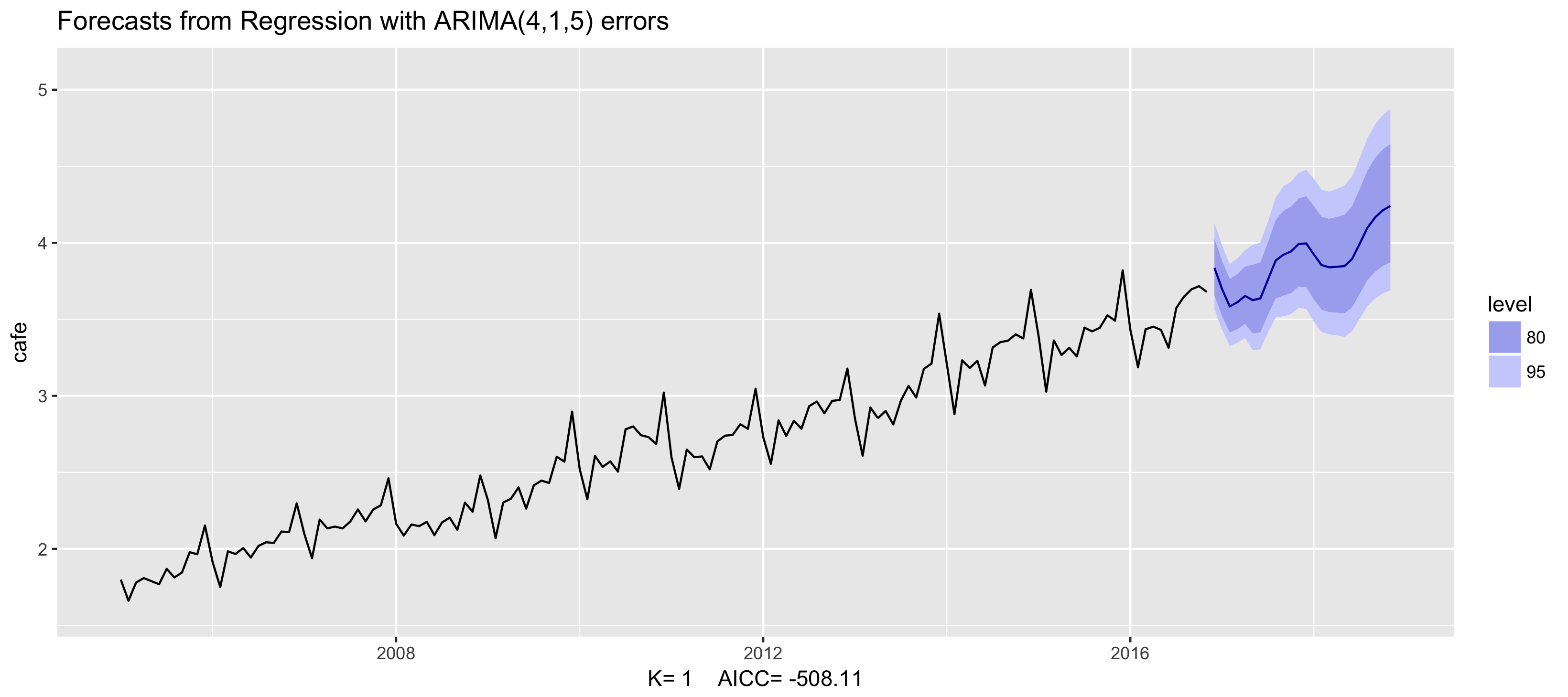
fit <- auto.arima(cafe, xreg = fourier(cafe, K = 1),
                  seasonal = FALSE, lambda = 0)
fit %>% forecast(xreg = fourier(cafe, K = 1, h = 24)) %>%
   autoplot() + ylim(1.6, 5.1)
例: オーストラリアのカフェ支出
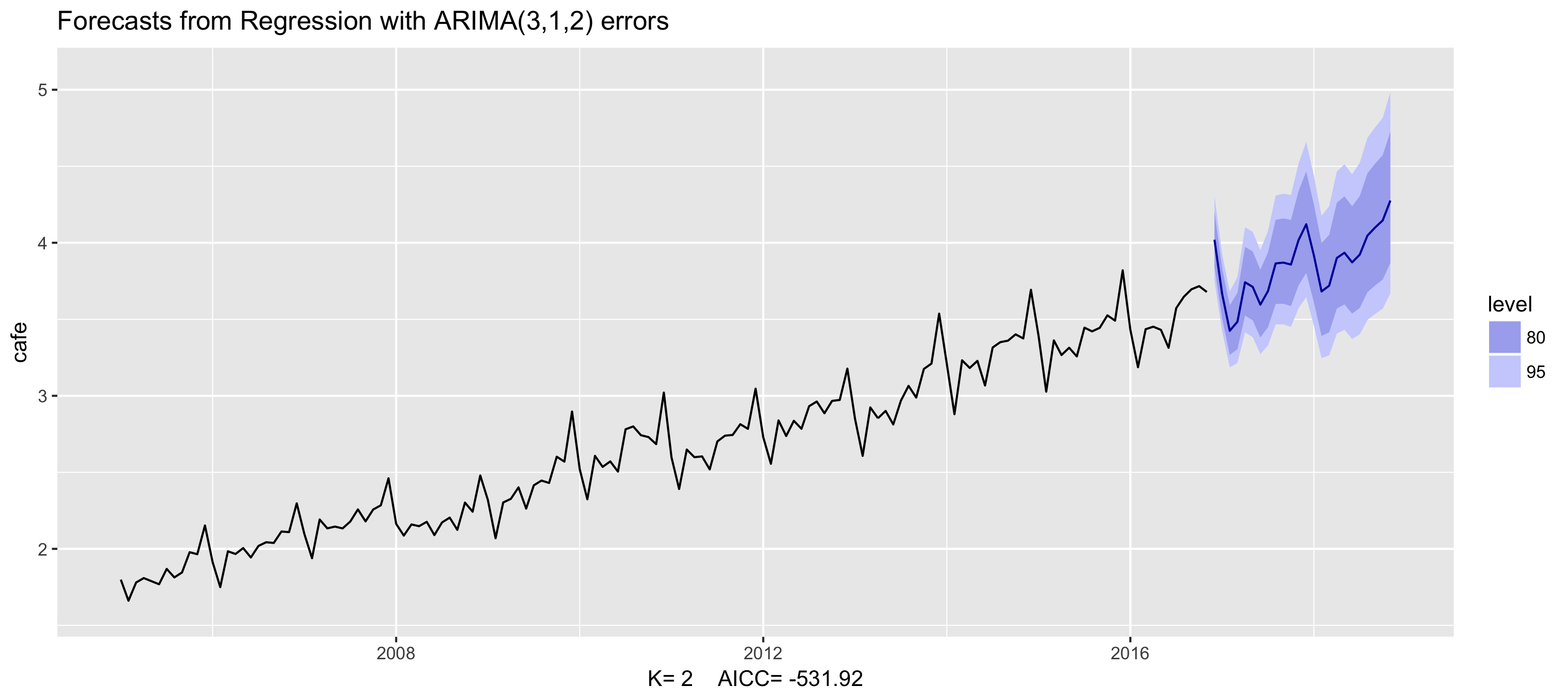
fit <- auto.arima(cafe, xreg = fourier(cafe, K = 2),
                  seasonal = FALSE, lambda = 0)
fit %>% forecast(xreg = fourier(cafe, K = 2, h = 24)) %>%
   autoplot() + ylim(1.6, 5.1)
例: オーストラリアのカフェ支出
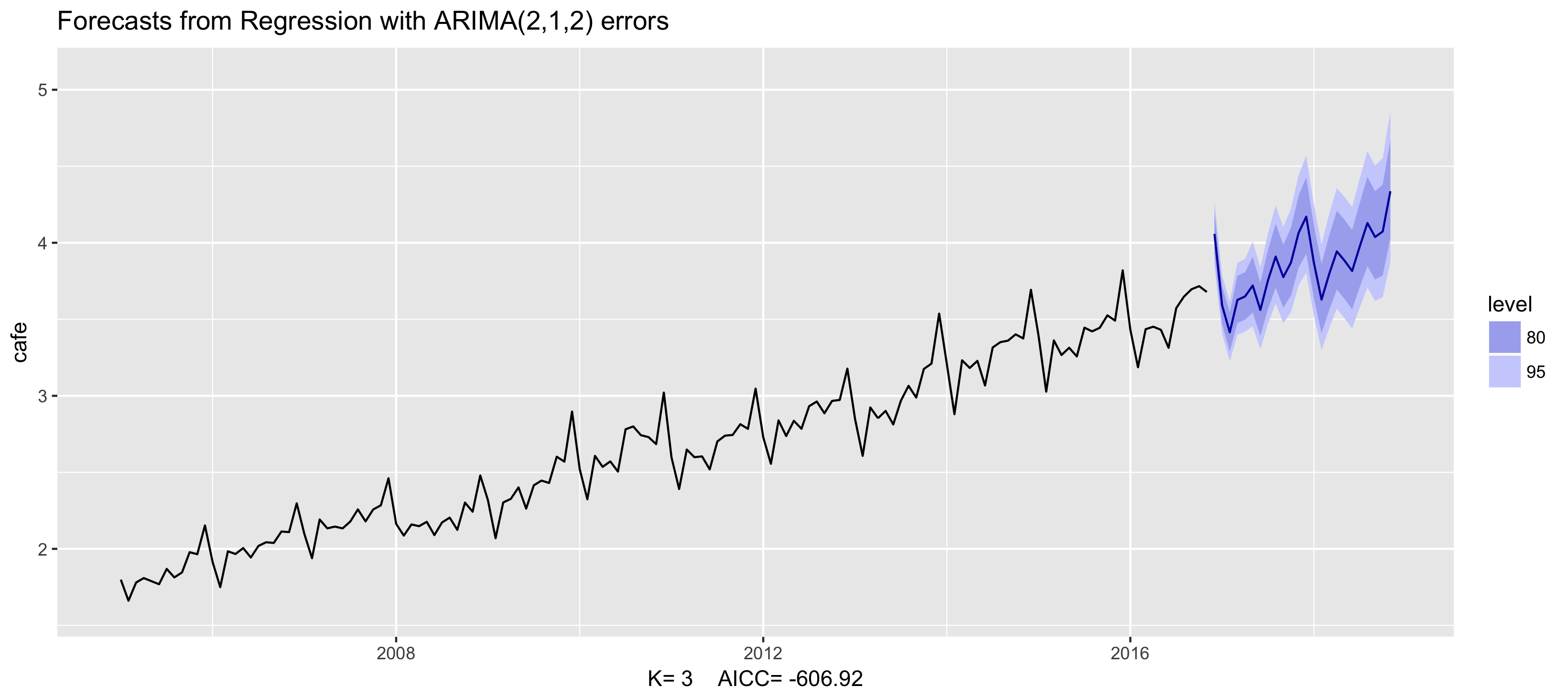
fit <- auto.arima(cafe, xreg = fourier(cafe, K = 3),
                  seasonal = FALSE, lambda = 0)
fit %>% forecast(xreg = fourier(cafe, K = 3, h = 24)) %>%
   autoplot() + ylim(1.6, 5.1)
例: オーストラリアのカフェ支出
fit <- auto.arima(cafe, xreg = fourier(cafe, K = 4),
                  seasonal = FALSE, lambda = 0)
fit %>% forecast(xreg = fourier(cafe, K = 4, h = 24)) %>%
   autoplot() + ylim(1.6, 5.1)
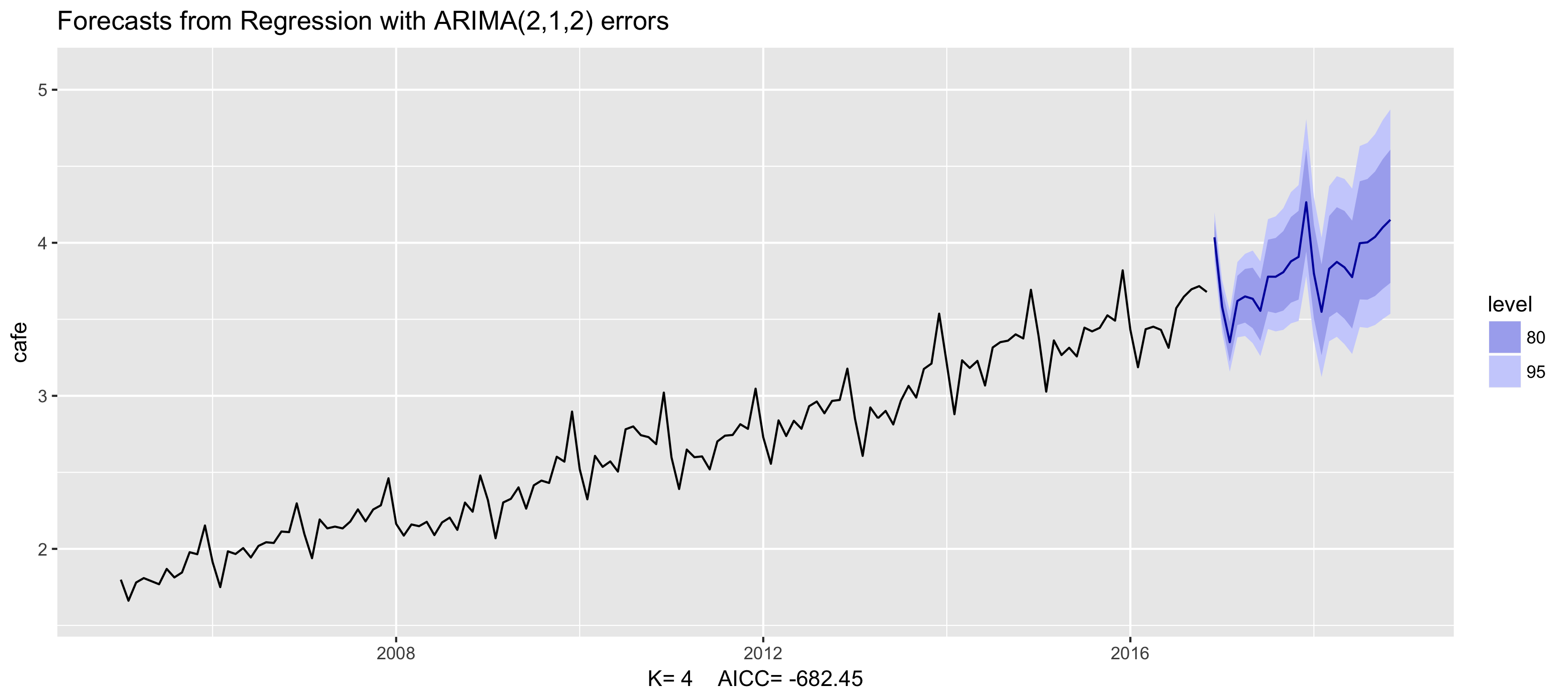
例: オーストラリアのカフェ支出
fit <- auto.arima(cafe, xreg = fourier(cafe, K = 5),
                  seasonal = FALSE, lambda = 0)
fit %>% forecast(xreg = fourier(cafe, K = 5, h = 24)) %>%
   autoplot() + ylim(1.6, 5.1)
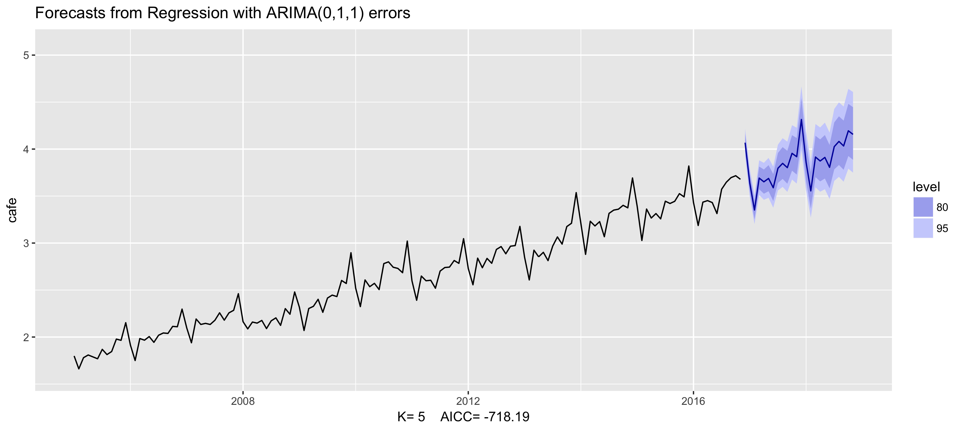
例: オーストラリアのカフェ支出
fit <- auto.arima(cafe, xreg = fourier(cafe, K = 6),
                  seasonal = FALSE, lambda = 0)
fit %>% forecast(xreg = fourier(cafe, K = 6, h = 24)) %>%
   autoplot() + ylim(1.6, 5.1)
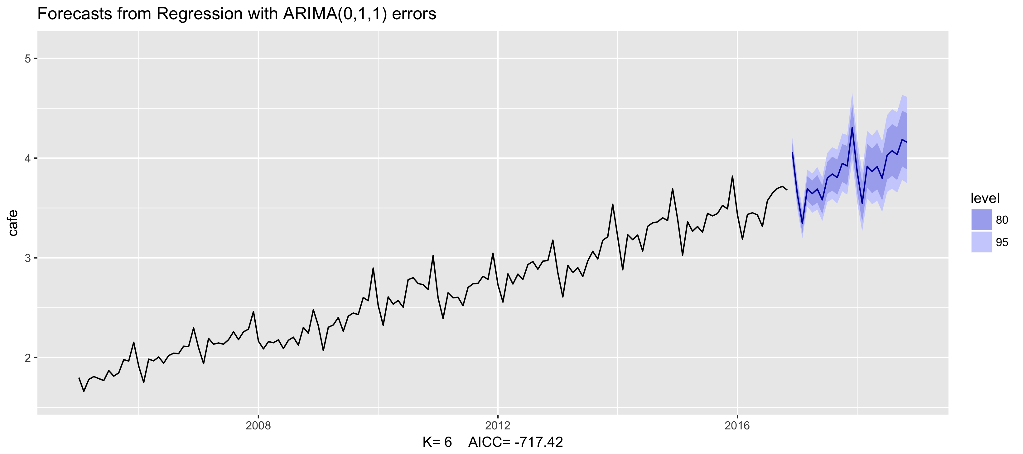
動的調和回帰

- 他の予測変数も追加可: $x_{t,1},...,x_{t,r}$
- $AIC_c$が最小となるKを選ぶ
- Kは m/2 を超えない
- 週次・日次・サブ日次データで有用

