共変量付き Weibull モデル

Pythonで学ぶSurvival Analysis

Shae Wang

Senior Data Scientist

生存関数の比較

Kaplan–Meier 推定量でグループ比較:

アパート vs. 戸建ての Kaplan–Meier 生存曲線。

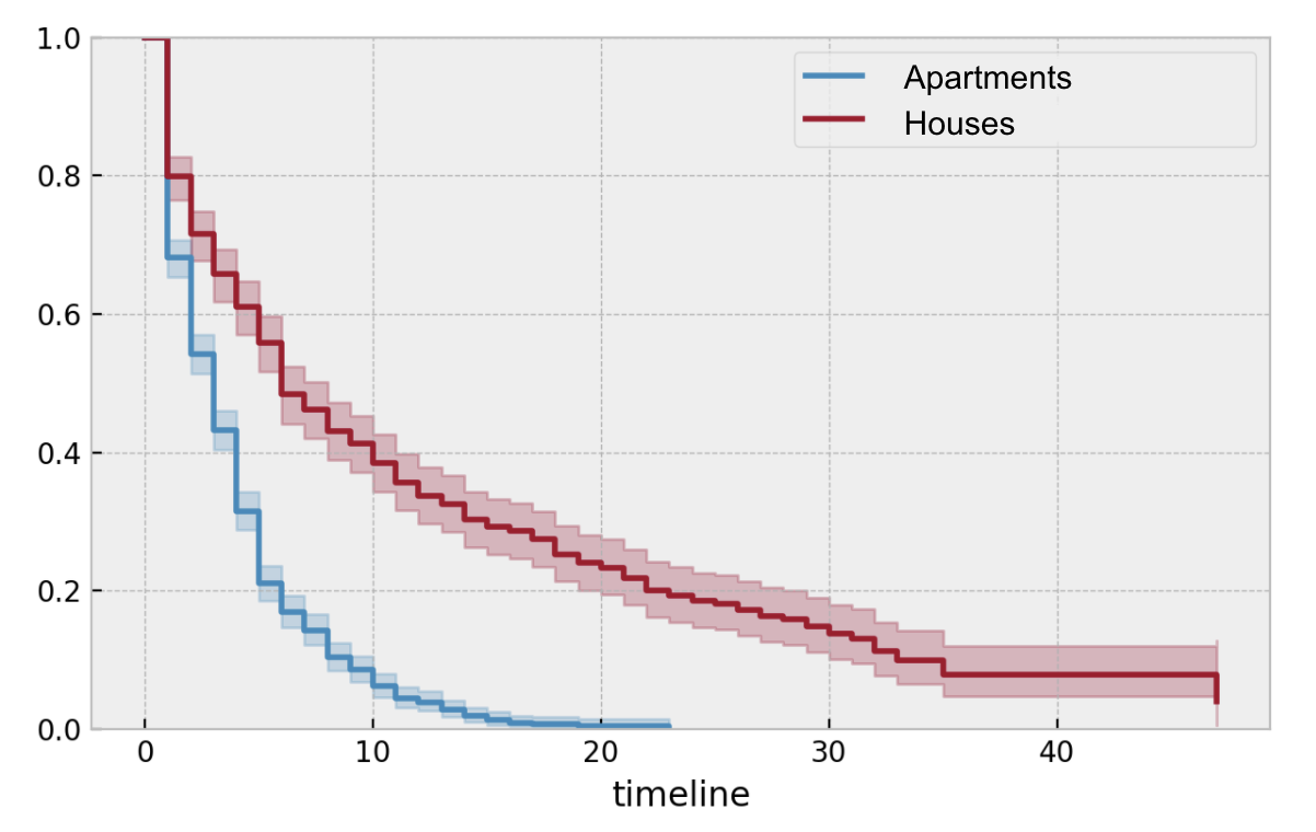
ログランク検定でグループ比較:

<lifelines.StatisticalResult: logrank_test>
 null_distribution = chi squared
degrees_of_freedom = 1
         test_name = logrank_test
 test_statistic    p  -log2(p)
           0.09 0.77      0.38

【Q】連続変数が生存関数に与える影響をどう評価するか？

生存回帰

共変量つきで生存関数をモデル化する手法
各共変量が生存関数に与える影響を定量化

$$Y_i=f(X_i,\beta)$$

$$Y_i: \text{duration}, X_i: \text{covariates}$$

例: 年齢、体重、国

Accelerated Failure Time (AFT) モデル

$$\text{集団 A}: S_A(t)$$

$$\text{集団 B}: S_B(t)$$

$$S_A(t)=S_B(t*\lambda)$$

$S_B(t)$ は $S_A(t)$ に沿って係数 $\lambda$ で加速/減速する。
AFT はこの加速/減速を共変量で表す。
共変量が $a$ から $b$ に変わると、イベント発生までの時間は加速率 $\lambda$ で変化。
例: $S_{dog}(t)=S_{human}(t*7)$

生存回帰のデータ

DataFrame 例: mortgage_df

id	property_type	principal	interest	property_tax	credit_score	duration	paid_off
1	house	1275	0.035	0.019	780	25	0
2	apartment	756	0.028	0.020	695	17	1
3	apartment	968	0.029	0.017	810	5	0
...	...	...	...	...	...	...	...
1000	house	1505	0.041	0.023	750	30	1

Weibull と AFT の統合: Weibull AFT モデル

DataFrame: mortgage_df
共変量:
- property_type はダミー変数に置換:
  - house: 「house」なら1、「apartment」なら0
- principal
- interest
- property_tax
- credit_score

WeibullAFTFitter クラスをインポート・生成

from lifelines import WeibullAFTFitter
aft = WeibullAFTFitter()

.fit() で学習

aft.fit(df=mortgage_df,
     duration_col="duration",
     event_col="paid_off")

モデル出力の解釈

print(aft.summary)

<lifelines.WeibullAFTFitter: fitted with 1808 observations, 340 censored>
                      coef  exp(coef)  se(coef)      z       p
lambda_ house         0.04       1.04      0.01   0.99    0.32  
        principal    -0.03       0.97      0.22  -1.04    0.30  
        interest      0.11       1.11      0.15   1.96    0.05  
        property_tax  0.31       1.36      0.27   1.15    0.25  
        credit_score -0.16       0.85      0.14  -2.33    0.02  
        Intercept     3.99      54.06      0.41   9.52 <0.0005   
rho_    Intercept     0.34       1.40      0.08   3.80 <0.0005

カスタム formula の WeibullAFTFitter

formula で共変量を指定:

aft.fit(df=mortgage_df,
        duration_col="duration",
        event_col="paid_off",
        formula="principal + interest * house")

相互作用をもつ線形モデルに相当:

$\beta_1$principal$+\beta_2$interest$+\beta_3$house$+\beta_4$interest$\cdot$house

モデル出力の解釈

print(aft.summary)

<lifelines.WeibullAFTFitter: fitted with 1808 observations, 340 censored>
                       coef  exp(coef)  se(coef)      z       p
lambda_ principal     -0.03       0.97      0.22  -1.04    0.30     
        interest       0.11       1.11      0.15   1.96    0.05  
        house          0.04       1.04      0.01   0.99    0.32  
        interest:house 0.06       1.06      0.14   0.42    0.64
        Intercept      3.99      54.06      0.41   9.52 <0.0005   
rho_    Intercept      0.34       1.40      0.08   3.80 <0.0005

Passons à la pratique !

Pythonで学ぶSurvival Analysis