縮小法

Rで学ぶ特徴量エンジニアリング

Jorge Zazueta

Research Professor and Head of the Modeling Group at the School of Economics, UASLP

一般的な正則化手法の2つ

Lasso

  • モデル係数の絶対値に比例する罰則を追加
  • 一部の係数を正確に0へ縮小
  • 対応する特徴量を実質的に除去
  • 自動特徴選択として使える

Ridge

  • 係数の二乗に比例する罰則を追加
  • Lassoのように係数を0にはしない
  • ただし過学習の抑制に有効
Rで学ぶ特徴量エンジニアリング

Lasso を試す

モデルを準備

recipe <- # レシピ定義
recipe(Loan_Status ~ ., data = train) %>%
  step_normalize(all_numeric_predictors()) %>% 
  step_dummy(all_nominal_predictors()) %>%
  update_role(Loan_ID, new_role = "ID")
# モデル設定
model_lasso_manual <- logistic_reg() %>%
  set_engine("glmnet") %>%
  set_args(mixture = 1, penalty = .2)
# ワークフローに束ねる
workflow_lasso_manual <-
  workflow() %>%
  add_model(model_lasso_manual) %>%
  add_recipe(recipe)

学習と確認

fit_lasso_manual <- # ワークフローを学習
  workflow_lasso_manual %>% 
  fit(train)
# 係数の確認
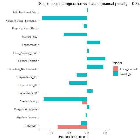
tidy(fit_lasso_manual)
# A tibble: 15 × 3
   term                    estimate penalty
   <chr>                      <dbl>   <dbl>
 1 (Intercept)               -0.816     0.2
 2 ApplicantIncome            0         0.2
 3 CoapplicantIncome          0         0.2
 4 LoanAmount                 0         0.2
 5 Loan_Amount_Term           0         0.2
 6 Credit_History            -0.220     0.2
 7 Gender_Female              0         0.2
 ...                          ...        ...
Rで学ぶ特徴量エンジニアリング

単純ロジスティック回帰 vs. Lasso

単純ロジスティック回帰とLassoの棒グラフ。

Rで学ぶ特徴量エンジニアリング

ハイパーパラメータのチューニング

チューニングありのモデル設定

model_lasso_tuned <- logistic_reg() %>%
  set_engine("glmnet") %>%
  set_args(mixture = 1, 
  penalty = tune()) 

workflow_lasso_tuned <-
  workflow() %>%
  add_model(model_lasso_tuned) %>%
  add_recipe(recipe)

penalty_grid <- grid_regular(
  penalty(range = c(-3, 1)),
  levels = 30)

チューニング結果の確認

tune_output <- tune_grid( 
  workflow_lasso_tuned,
  resamples = vfold_cv(train, v = 5),
  metrics = metric_set(roc_auc),
  grid = penalty_grid)
autoplot(tune_output)
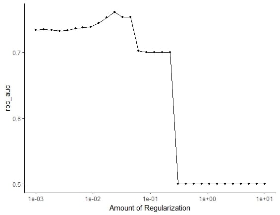
ROC_AUC と正則化量の関係を示すチャート。

Rで学ぶ特徴量エンジニアリング

結果の確認

自動選択された特徴量

best_penalty <- 
select_by_one_std_err(tune_output, 
metric = 'roc_auc', desc(penalty)) 

# 最終モデルの学習
final_fit<- 
finalize_workflow(workflow_lasso_tuned, 
best_penalty) %>%
  fit(data = train)
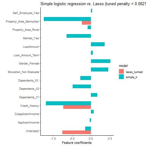
final_fit_se %>% tidy()
# A tibble: 15 × 3
   term                    estimate penalty
   <chr>                      <dbl>   <dbl>
 1 (Intercept)               -0.660  0.0452
 2 ApplicantIncome            0      0.0452
 3 CoapplicantIncome          0      0.0452
 4 LoanAmount                 0      0.0452
 5 Loan_Amount_Term           0      0.0452
 6 Credit_History            -0.948  0.0452
 7 Gender_Female              0      0.0452
 8 Married_Yes               -0.191  0.0452
 9 Dependents_X1              0      0.0452
10 Dependents_X2              0      0.0452
11 Dependents_X3.             0      0.0452
12 Education_Not.Graduate     0      0.0452
13 Self_Employed_Yes          0      0.0452
14 Property_Area_Rural        0      0.0452
15 Property_Area_Semiurban   -0.163  0.0452
Rで学ぶ特徴量エンジニアリング

単純ロジスティック回帰 vs. チューニング済みLasso

Rで学ぶ特徴量エンジニアリング

Ridge 正則化

mixture = 0 のとき Ridge

model_ridge_tuned <- logistic_reg() %>%
  set_engine("glmnet") %>%
  set_args(mixture = 0, penalty = tune()) 

workflow_ridge_tuned <-
  workflow() %>%
  add_model(model_ridge_tuned) %>%
  add_recipe(recipe)

tune_output <- tune_grid( 
  workflow_ridge_tuned,
  resamples = vfold_cv(train, v = 5),
  metrics = metric_set(roc_auc),
  grid = penalty_grid)
tune_output <- tune_grid( 
  workflow_ridge_tuned,
  resamples = vfold_cv(train, v = 5),
  metrics = metric_set(roc_auc),
  grid = penalty_grid)  
 autoplot(tune_output)
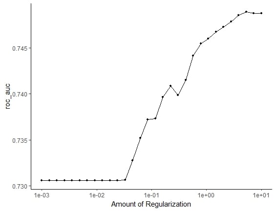
Rで学ぶ特徴量エンジニアリング

Ridge 正則化

best_penalty <- 
select_by_one_std_err(tune_output,
metric = 'roc_auc', desc(penalty)) 
best_penalty

final_fit<- 
finalize_workflow(workflow_ridge_tuned, 
best_penalty) %>%
  fit(data = train)
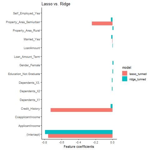
tidy(final_fit)
# A tibble: 15 × 3
   term                      estimate penalty
   <chr>                        <dbl>   <dbl>
 1 (Intercept)             -0.799          10
 2 ApplicantIncome          0.00232        10
 3 CoapplicantIncome        0.0000537      10
 4 LoanAmount               0.00291        10
 5 Loan_Amount_Term         0.00161        10
 6 Credit_History          -0.0245         10
 7 Gender_Female            0.00850        10
 8 Married_Yes             -0.0140         10
 9 Dependents_X1            0.00497        10
10 Dependents_X2           -0.0100         10
11 Dependents_X3.           0.00259        10
12 Education_Not.Graduate   0.00308        10
13 Self_Employed_Yes        0.00892        10
14 Property_Area_Rural      0.0109         10
15 Property_Area_Semiurban -0.0139         10
Rで学ぶ特徴量エンジニアリング

Ridge と Lasso の比較

Rで学ぶ特徴量エンジニアリング

練習しましょう!

Rで学ぶ特徴量エンジニアリング

Preparing Video For Download...