ドメイン知識で新しい特徴量を作成する

Rで学ぶ特徴量エンジニアリング

Jorge Zazueta

Research Professor and Head of the Modeling Group at the School of Economics, UASLP

ドメイン知識の重要性

ドメイン知識により、特定のモデルや課題に有用な特徴量を見つけて作れます。

特徴量エンジニアリングは、既存データから新たな入力特徴量を作ることです。

■ ドメイン知識の例:

金融: 破産の主要因
医療: 特定治療に関連する既往症
マーケティング: 消費者セグメントの識別要因

実務経験に基づく変数作成

次の特徴量ベクトルに基づき、ホテルのキャンセルを予測します。

features <- 
c("IsCanceled", "LeadTime",
  "arrival_date",
  "StaysInWeekendNights",
  "StaysInWeekNights",
  "PreviousCancellations",
  "PreviousBookingsNotCanceled",
  "ReservedRoomType",
  "AssignedRoomType","BookingChanges",
  "DepositType","CustomerType",
  "ADR","TotalOfSpecialRequests")

■ 生データからの特徴量

arrival_date から有益な特徴量を生成できます。

到着日は曜日・週・月・祝日などに分解できる

ただし手作業はすぐ煩雑になります。自動化が必要です。

tidymodels フレームワーク

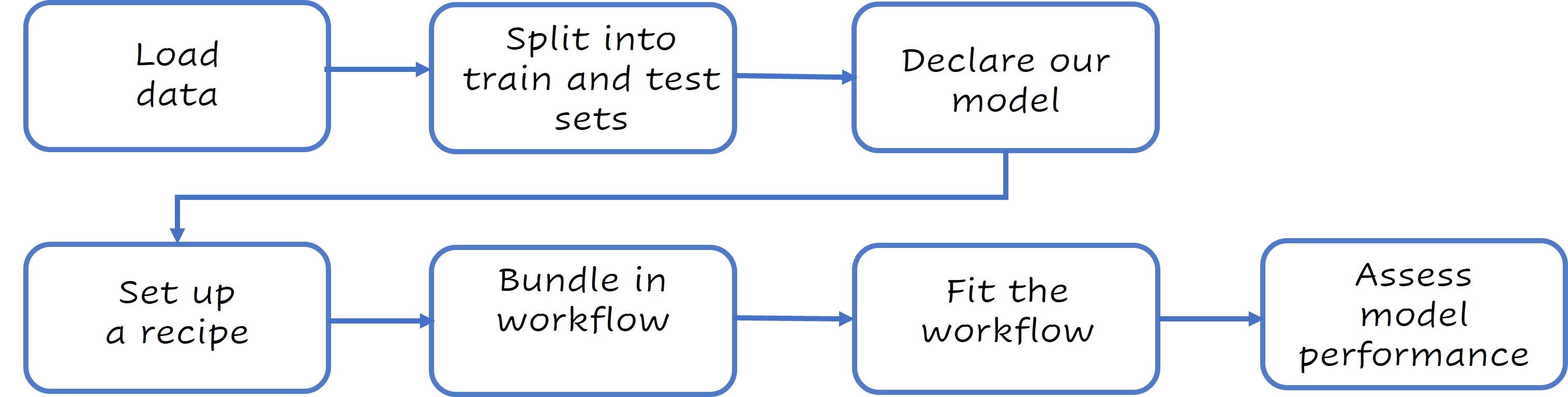
tidymodels（tidyverse の原則に基づくモデリング/機械学習パッケージ群）を使い、特徴量エンジニアリングを重視したワークフローで進めます。

シンプルな tidymodels ワークフロー: データ読み込み、モデル宣言、データ分割、レシピ設定、ワークフローに束ねる、学習、性能評価。

詳しくは www.tidymodels.org を参照してください。

¹ [Tidyverse の指針](https://design.tidyverse.org/unifying-principles.html)

分析に向けたデータ準備

まずはデータ準備から始めます。

cancelations <- 
  cancelations %>% 
  mutate(across(where(is_character),as.factor))

set.seed(123)
split <- cancellations %>% 
    initial_split(
    strata = "IsCanceled")
train <- training(split)
test <- testing(split)

prop パラメータで学習/テストの分割比を変更できます（既定は 3/4）。

initial_split(data, prop = 3/4, strata = NULL)

train と test が同様のキャンセル比率か確認します。

train %>% 
  select(IsCanceled) %>% table() %>% 
  prop.table()

IsCanceled
        0         1 
0.5826946 0.4173054

test %>% 
  select(IsCanceled) %>% table() %>% 
  prop.table()

IsCanceled
        0         1 
0.5827788 0.4172212

ワークフローの構築

モデルを宣言

lr_model <- logistic_reg()

レシピを作成

lr_recipe <- 
  recipe(IsCanceled ~., data = train) %>%
  update_role(Agent, new_role = "ID" ) %>%
  step_date(arrival_date, 
      features = c("dow", "week", "month")) %>%
  step_holiday(arrival_date, 
      holidays = timeDate::listHolidays("US")) %>%
  step_rm(arrival_date) %>%
  step_dummy(all_nominal_predictors())

lr_recipe を出力

DNT_CURLY_TAG_3

Recipe

Inputs:
      role #variables
        ID          1
   outcome          1

 predictor         13

Operations:
Date features from arrival_date
Holiday features from arrival_date
Variables removed arrival_date
Dummy variables from all_nominal_predictors()

ワークフローの構築

モデルとレシピを workflow にまとめます。

lr_workflow <- 
  workflow()%>%
  add_model(lr_model)%>%
  add_recipe(lr_recipe)

ワークフローを学習

lr_fit <- 
  lr_workflow %>%
  fit(data = train)

ワークフローの構築

tidy(lr_fit) でモデル要約を確認できます。

# A tibble: 65 × 5
   term                        estimate std.error statistic   p.value
   <chr>                          <dbl>     <dbl>     <dbl>     <dbl>
 1 (Intercept)                 -1.92     0.228        -8.43 3.57e- 17
 2 LeadTime                     0.00414  0.000268     15.4  1.16e- 53
 3 StaysInWeekendNights         0.0860   0.0382        2.25 2.45e-  2
 4 StaysInWeekNights            0.0804   0.0185        4.34 1.40e-  5
 5 PreviousCancellations        2.39     0.147        16.2  2.45e- 59
 6 PreviousBookingsNotCanceled -0.440    0.0450       -9.77 1.45e- 22
 7 BookingChanges              -0.449    0.0463       -9.69 3.18e- 22
 8 ADR                          0.0104   0.000782     13.2  4.85e- 40
 9 TotalOfSpecialRequests      -0.727    0.0316      -23.0  5.29e-117
10 arrival_date_week            0.0245   0.0171        1.43 1.53e-  1
# … with 55 more rows
# ℹ Use `print(n = ...)` to see more rows

モデル性能の評価

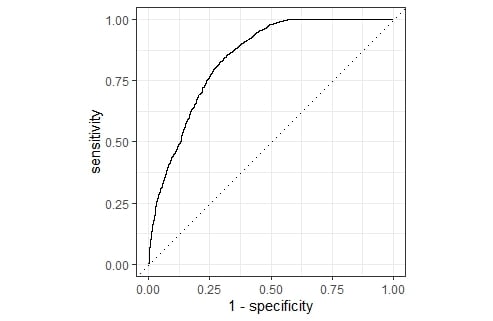
モデル性能を評価します。

lr_aug <- lr_fit %>% augment(test)

bind_rows(
  lr_aug %>% 
  roc_auc(truth = IsCanceled,.pred_0),
  lr_aug %>% 
  accuracy(truth = IsCanceled,.pred_class))

# A tibble: 2 × 3
  .metric  .estimator .estimate
  <chr>    <chr>          <dbl>
1 roc_auc  binary         0.842
2 accuracy binary         0.782

lr_aug %>%
  roc_curve(truth = IsCanceled, .pred_0) %>%
  autoplot()

本モデルのROC曲線。

練習してみましょう！

Rで学ぶ特徴量エンジニアリング