次元削減

Rで学ぶ特徴量エンジニアリング

Jorge Zazueta

Research Professor and Head of the Modeling Group at the School of Economics, UASLP

分散ゼロの特徴量

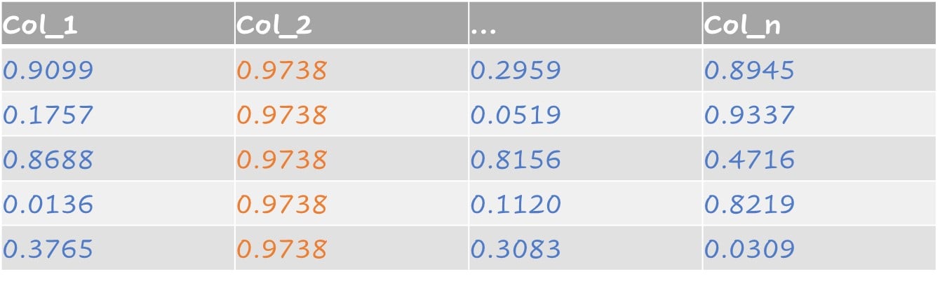
一部のデータセットには定数列、つまり分散ゼロの列があります。recipe() に step_zv() を追加して、これらの特徴量を除外できます。

分散ゼロの特徴量を示す表。

ほぼゼロ分散の特徴量

ほぼゼロ分散の特徴量には、単一の値しか持たない予測子に加えて、次の両方の性質を持つ予測子が含まれます。

サンプル数に比べて一意の値が非常に少ない
最頻値の出現頻度と2番目に多い値の出現頻度の比が大きい

ほぼゼロ分散の例:

100件の観測で値は2種類だが、そのうち1つは1回しか出ない。

step_nzv() は、これらの性質を持つ予測子を特定して除去します。

主成分分析（PCA）

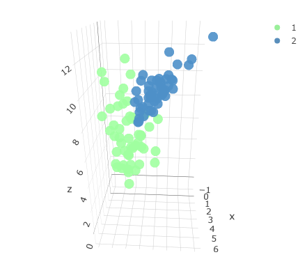
2つのクラスを持つ元の3次元データセット。

2つのデータクラスを示す3次元グラフ。

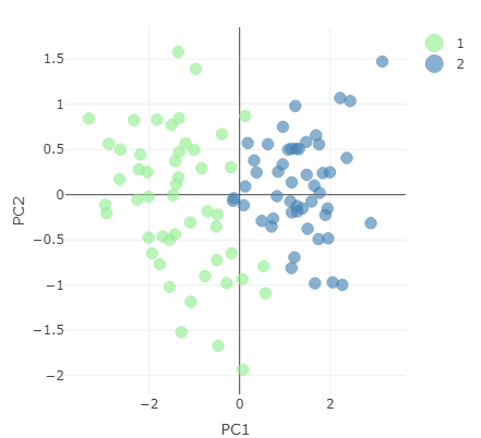
最初の2つの主成分で表現した縮約データセット。

最初の2つの主成分の散布図として2つのデータクラスを示す2次元グラフ。

recipe を準備しましょう

PCA を行う recipe を作成し、prep() で出力を取得します。

pc_recipe <- 
recipe(~., data = loans_num) %>%
  step_nzv(all_numeric()) %>%
  step_normalize(all_numeric()) %>%
  step_pca(all_numeric())

pca_output <- prep(pc_recipe)

pca_output に対して names() を呼ぶと、利用可能な情報を確認できます。

names(pca_output)

 [1] "var_info"       "term_info"     
 [3] "steps"          "template"      
 [5] "levels"         "retained"      
 [7] "requirements"   "tr_info"       
 [9] "orig_lvls"      "last_term_info"

説明分散を見つける

pca_output オブジェクトから標準偏差を取り出し、説明分散を計算します。

stdv <- pca_output$steps[[3]]$res$sdev

var_explained <- stdv^2/sum(stdv^2)

PCA = tibble(PC = 1:length(stdv),
          var_explained = var_explained, 
          cumulative = cumsum(var_explained))

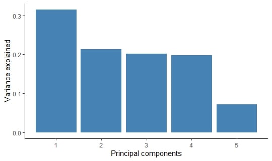
主成分ごとの説明分散を示す表。

# A tibble: 5 × 3
     PC var_explained cumulative
  <int>         <dbl>      <dbl>
1     1        0.315       0.315
2     2        0.214       0.529
3     3        0.202       0.730
4     4        0.198       0.928
5     5        0.0722      1

説明分散を可視化する

出力を ggplot2 で棒グラフにします。

PCA %>% 
ggplot(aes(x = PC, 
           y = var_explained)) +
  geom_col(fill = "steelblue") +
  xlab("Principal components") +
  ylab("Variance explained")

主成分ごとの説明分散。

主成分ごとの説明分散を示す棒グラフ。

Passons à la pratique !

Rで学ぶ特徴量エンジニアリング