生データの情報量を高める

Rで学ぶ特徴量エンジニアリング

Jorge Zazueta

Research Professor and Head of the Modeling Group at the School of Economics, UASLP

生データへの対処

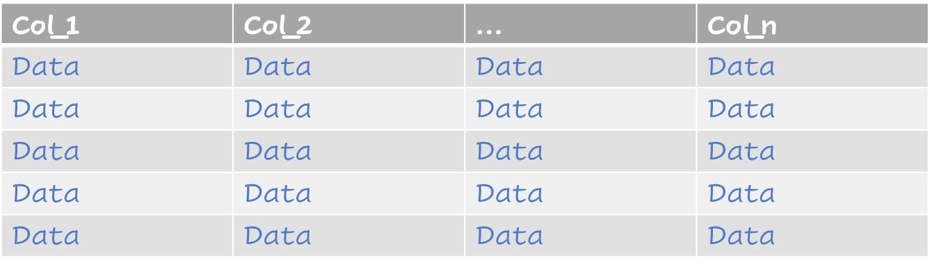
欠損値を含む一般的なデータセット
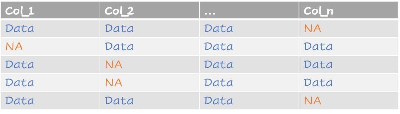
欠損データの例を示す表

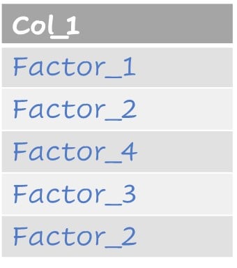
値を因子として扱う

因子型データの例を示す表

Rで学ぶ特徴量エンジニアリング

生データへの対処

補完後のデータセット

補完後で欠損がない表

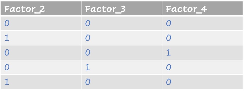
因子をダミー変数で表現

因子をダミー変数で表現

Rで学ぶ特徴量エンジニアリング

ローンデータセット

# A tibble: 614 × 13
   Loan_ID  Gender Married Dependents Educa…¹ Self_…² Appli…³ Coapp…⁴ LoanA…⁵ Loan_…⁶
   <fct>    <fct>  <fct>   <fct>      <fct>   <fct>     <dbl>   <dbl>   <dbl>   <dbl>
 1 LP001002 Male   No      0          Gradua… No         5849       0      NA     360
 2 LP001003 Male   Yes     1          Gradua… No         4583    1508     128     360
 3 LP001005 Male   Yes     0          Gradua… Yes        3000       0      66     360
 4 LP001006 Male   Yes     0          Not Gr… No         2583    2358     120     360
 5 LP001008 Male   No      0          Gradua… No         6000       0     141     360
 6 LP001011 Male   Yes     2          Gradua… Yes        5417    4196     267     360
 7 LP001013 Male   Yes     0          Not Gr… No         2333    1516      95     360
 8 LP001014 Male   Yes     3+         Gradua… No         3036    2504     158     360
 9 LP001018 Male   Yes     2          Gradua… No         4006    1526     168     360
10 LP001020 Male   Yes     1          Gradua… No        12841   10968     349     360
# … with 604 more rows, 3 more variables: Credit_History <dbl>, Property_Area <fct>,
#   Loan_Status <fct>, and abbreviated variable names ¹​Education, ²​Self_Employed,
#   ³​ApplicantIncome, ⁴​CoapplicantIncome, ⁵​LoanAmount, ⁶​Loan_Amount_Term
# ℹ Use `print(n = ...)` to see more rows, and `colnames()` to see all variable names
Rで学ぶ特徴量エンジニアリング

欠損値

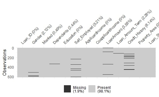
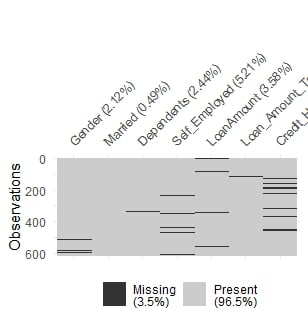
パッケージ naniarvis_miss(loans) で、loans の欠損を可視化できます。

データセット全体の欠損を示すグラフ。

Rで学ぶ特徴量エンジニアリング

欠損値

欠損のある列だけを選べば、表を拡大して確認できます。

loans %>% 
select(Gender, 
       Married, 
       Dependents,
       Self_Employed,
       LoanAmount,
       Loan_Amount_Term, 
       Credit_History) %>%
  vis_miss()

欠損値を詳しく見る

選択した特徴量の欠損値を示すグラフ。

Rで学ぶ特徴量エンジニアリング

欠損値とダミー変数

同じレシピ内で、欠損値補完とダミー変数化を行えます。

lr_recipe <- 
  recipe(Loan_Status ~., 
         data = train) %>%
  update_role(Loan_ID, 
              new_role = "ID" ) %>%
  step_impute_knn(all_predictors()) %>%
  step_dummy(all_nominal_predictors())

レシピを表示

lr_recipe
Recipe

Inputs:

      role #variables
        ID          1
   outcome          1
 predictor         30

Operations:

K-nearest neighbor imputation for all_predictors()
Dummy variables from all_nominal_predictors()
Rで学ぶ特徴量エンジニアリング

適切なレシピ手順を探す

他の補完手法や全レシピ手順は、tidymodels ドキュメント www.tidymodels.org/find/recipes で確認できます。
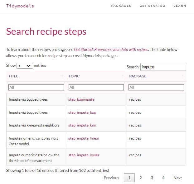
tidymodels ドキュメント内のレシピ検索ツール。

Rで学ぶ特徴量エンジニアリング

モデルの学習と評価

# Fit
lr_fit <- 
  lr_workflow %>% fit(data = train)
lr_aug <- 
  lr_fit %>% augment(test)
# Assess
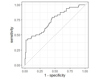
lr_aug %>%
  roc_curve(truth = Loan_Status, .pred_N) %>%
  autoplot()

bind_rows(lr_aug %>%
            roc_auc(truth = Loan_Status,
                    .pred_N),
          lr_aug %>%
            accuracy(truth = Loan_Status,
                     .pred_class))
# A tibble: 2 × 3
  .metric  .estimator .estimate
  <chr>    <chr>          <dbl>
1 roc_auc  binary         0.738
2 accuracy binary         0.792
Rで学ぶ特徴量エンジニアリング

練習してみましょう!

Rで学ぶ特徴量エンジニアリング

Preparing Video For Download...