検証済みGARCHモデルを本番運用する

Rで学ぶGARCHモデル

Kris Boudt

Professor of finance and econometrics

本番での利用

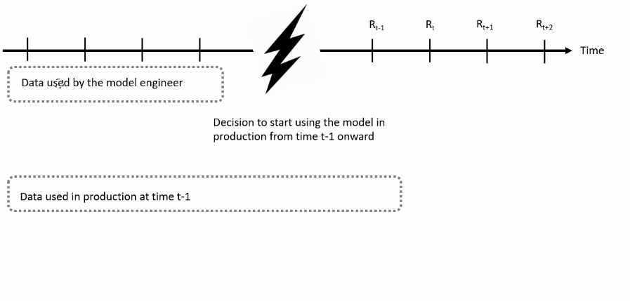
年ごとの日次リターンの分布

新機能

ugarchfilter()で直近の平均とボラティリティの動学を分析
予測にはugarchforecast()をugarchspec（ugarchfit()ではなく）に適用

MSFTリターンの例

msftret: 1999〜2017の営業日リターン。
モデル当てはめは2010年末までのリターンで実施したとします。
2017年末にこのモデルで過去のボラティリティ動学を分析し、将来のボラティリティを予測します。

手順1：最終モデル仕様を定義

2010年末時点のmsftretで最良モデルを当てはめます。

# Specify AR(1)-GJR GARCH model with skewed student t distribution
garchspec <- ugarchspec(mean.model = list(armaOrder = c(1,0)),
 variance.model = list(model = "gjrGARCH"), distribution.model = "sstd")
# Estimate the model
garchfit <- ugarchfit(data = msftret["/2010-12"], spec = garchspec)

本番用仕様progarchspecを定義し、setfixed(progarchspec) <- as.list(coef(garchfit))を実行します。

progarchspec <- garchspec
setfixed(progarchspec) <- as.list(coef(garchfit))

手順2：平均とボラティリティ動学の分析

ugarchfilter()を使用します。

garchfilter <- ugarchfilter(data = msftret, spec = progarchspec)
plot(sigma(garchfilter))

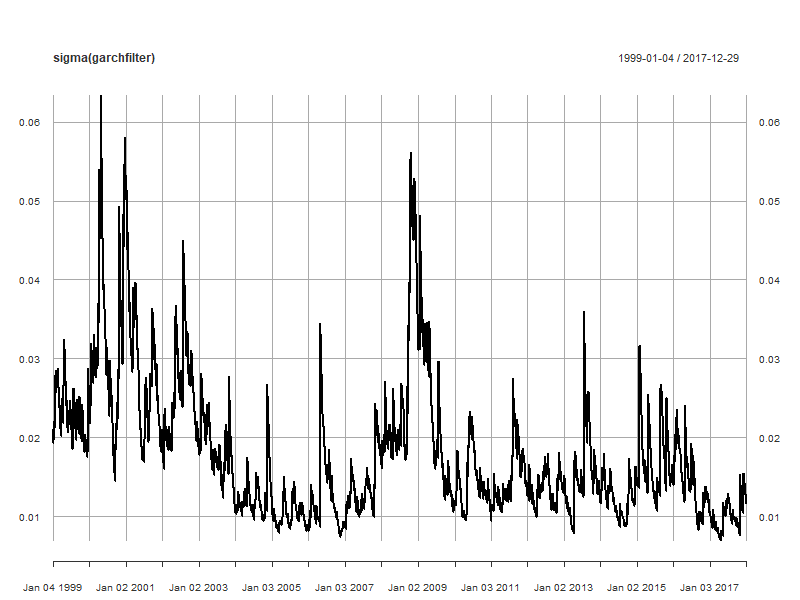
年ごとの日次リターンの分布

手順3：将来リターンを予測する

garchforecast <- ugarchforecast(data = msftret,
                                fitORspec = progarchspec, 
                                n.ahead = 10) # Make predictions for next ten days

cbind(fitted(garchforecast), sigma(garchforecast))

       2017-12-29 2017-12-29
T+1  0.0004781733 0.01124870
T+2  0.0003610470 0.01132550
T+3  0.0003663683 0.01140171
T+4  0.0003661265 0.01147733
T+5  0.0003661375 0.01155238
T+6  0.0003661370 0.01162688
T+7  0.0003661371 0.01170083
T+8  0.0003661371 0.01177424
T+9  0.0003661371 0.01184712
T+10 0.0003661371 0.01191948

シミュレーションでの利用

観測リターンの分析に完全モデルを当てる代わりに、人工的な対数リターンをシミュレーションできます。

$$ r_{t} = \log(P_{t}) - \log(P_{t-1}) $$

将来リターンの不確実性と価格への影響を評価するのに有用です。将来価格は次の通り：

$$ P_{t + h} = P_{t} \exp(r_{t + 1} + r_{t + 2} + \ldots + r_{t + h}) $$

手順1：シミュレーションモデルを較正する

推定には対数リターンを使用します。

# Compute log returns
msftlogret <- diff(log(MSFTprice))[-1]

モデルを推定し、その推定値をシミュレーションモデルに設定します。

garchspec <- ugarchspec(mean.model = list(armaOrder = c(1, 0)),
                        variance.model = list(model = "gjrGARCH"),
                        distribution.model = "sstd")
# Estimate the model
garchfit <- ugarchfit(data = msftlogret, spec = garchspec)

# Set that estimated model as the model to be used in the simulation
simgarchspec <- garchspec
setfixed(simgarchspec) <- as.list(coef(garchfit))

手順2：`ugarchpath()`でシミュレーションを実行

ugarchpath() によるシミュレーションでは次を指定します：

spec：完全に指定したGARCHモデル
m.sim：生成するシミュレーション系列の本数
n.sim：各系列の観測数（例：252）
rseed：乱数の種（再現性のため）

simgarch <- ugarchpath(spec = simgarchspec, m.sim = 4,
                       n.sim = 10 * 252, rseed = 12345)

手順3：シミュレーションリターンの分析

fitted() でシミュレーションリターンを取得します。

simret <- fitted(simgarch)
plot.zoo(simret)

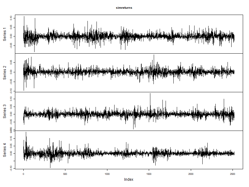
シミュレーションしたリターン

シミュレーションボラティリティの分析

plot.zoo(sigma(simgarch))

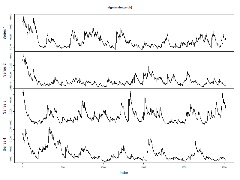
シミュレーションしたボラティリティ

シミュレーション価格の分析

初期価格1として、株価の10年シミュレーションを4本描画します。

simprices <- exp(apply(simret, 2, "cumsum"))
matplot(simprices, type = "l", lwd = 3)

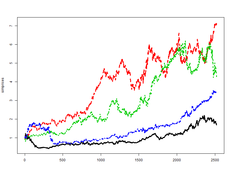
シミュレーションした価格

setfixed(), ugarchfilter(), ugarchforecast(), ugarchpath()で演習の時間です

Rで学ぶGARCHモデル