ggplot2 を使った R でのグラフ可視化

SAS ユーザーのための R

Melinda Higgins, PhD

Research Professor/Senior Biostatistician Emory University

ggplot2 パッケージ

ggplot2 の六角形ロゴ

ggplot2 は R 向けの強力なグラフィックスパッケージです
ggplot の「GG」は「グラフィックスの文法」を意味します
ggplot2 はレイヤーを重ねてグラフィックスを構築します
ベースとなるグラフィックスレイヤーに1つ以上の幾何オブジェクトを追加します

レイヤー - ベースレイヤー

# Create plot for x=sex and y=diameter
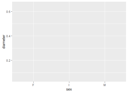
ggplot(data = abalone, aes(sex, diameter))

ggplot() でベースレイヤーを定義します
data = abalone を設定します
aes に sex と diameter を設定します
プロットにはまだ描画オブジェクトがありません
x軸は sex の準備ができています
y軸は diameter の準備ができています
グリッドが配置されます

ggplot2 のグラフ環境（ボックスプロットなし）

レイヤー - ボックスプロットの geom を追加

# Add boxplot geometric object or geom
ggplot(data = abalone,
       aes(sex, diameter)) +
  geom_boxplot()

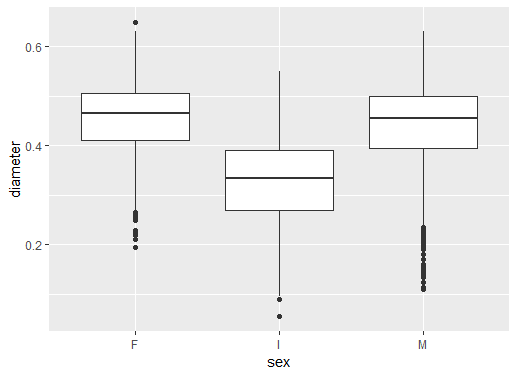
演算子 + でレイヤーを追加します
ボックスプロット geom_boxplot() を追加しました
結果は複数のボックスプロットになります
性別ごとのアワビの直径
F はメス、I は幼体、M はオスを表します

ggplot2 にボックスプロットを追加

レイヤー - テーマを追加

# Add black white theme
ggplot(data = abalone,
       aes(sex, diameter)) +
  geom_boxplot() +
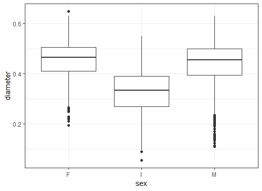
  theme_bw()

theme_bw() を使って「テーマ」レイヤーを追加します
灰色の背景を削除します
プロットの周りに黒枠を描画します

ggplot2 ボックスプロットに白黒テーマを追加

ボックスプロットの geom をバイオリンの geom に変更

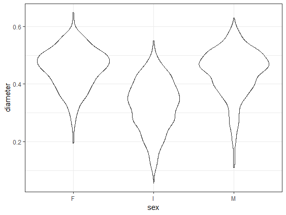
# Change to geom_violin()
ggplot(data = abalone,
       aes(sex, diameter)) +
  geom_violin() +
  theme_bw()

geom_violin が geom_boxplot を置き換えます
バイオリンに似た形を作成します
データの密度分布を反映します
簡単な変更で新しい図が作成できます

ggplot2 バイオリンプロット

単一変数のヒストグラム

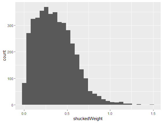
# Make histogram of shuckedWeight
ggplot(abalone, aes(shuckedWeight)) +
  geom_histogram()

1つの変数のヒストグラムを作成します
変数1つに対して aesthetic は1つです
geom_histogram() を追加します
aes() に shuckedWeight を設定します
デフォルトの色は変更が必要です

ggplot2 の全体が黒いヒストグラム

ヒストグラムに色を追加

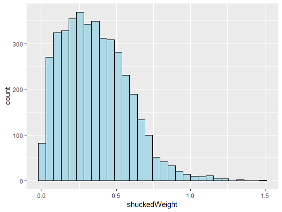
# Make lines black and fill light blue
ggplot(abalone, aes(shuckedWeight)) +
  geom_histogram(color = "black",
                 fill = "lightblue")

グラフィックパラメータを変更します
ビンの線の color を設定します
ビンの fill カラーを設定します
各オプションは () の中に設定します
ヒストグラムの見た目が良くなりました

ggplot2 の青いバーと黒い枠線のヒストグラム

ヒストグラムにタイトルと軸ラベルを追加

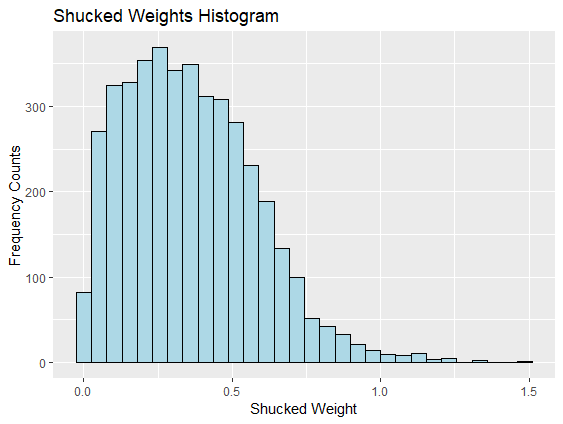
# Add x, y axis labels and title
ggplot(abalone, aes(shuckedWeight)) +
  geom_histogram(color = "black",
                 fill = "lightblue") +
  xlab("Shucked Weight") +
  ylab("Frequency Counts") +
  ggtitle("Shucked Weights Histogram")

軸ラベルとタイトルをより分かりやすくします
軸には xlab() と ylab() を使います
タイトルには ggtitle() を使います
この図はこのまま公開できます！

ggplot2 の軸ラベルとタイトルを追加したヒストグラム

散布図を作成

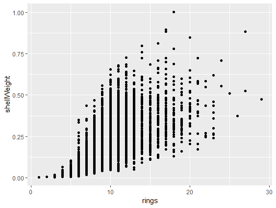
# Make scatterplot with geom_point()
ggplot(abalone,
       aes(rings, shellWeight)) +
  geom_point()

散布図の aes には2つの変数が必要です
geom_point() で点を追加します
輪数ごとの殻重量の散布図

ggplot2 の輪数ごとの殻重量の散布図

散布図に平滑化フィット線を追加

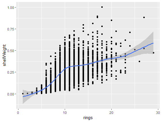
# Add smoothed fit line
ggplot(abalone,
       aes(rings, shellWeight)) +
  geom_point() +
  geom_smooth()

散布図に geom_smooth() の線を追加します
網掛けの信頼区間を含みます

ggplot2 の平滑化フィット線を追加した散布図

別の変数でパネルを作成

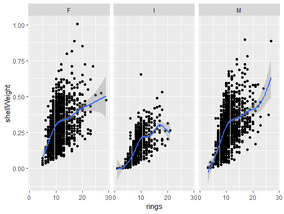
# Add panels using facet_wrap()
ggplot(abalone,
       aes(rings, shellWeight)) +
  geom_point() +
  geom_smooth() +
  facet_wrap(vars(sex))

散布図にもう1つレイヤーを追加します
アワビの性別ごとにパネルを作成します
facet_wrap() レイヤーを追加します
vars(sex) でパネルの変数を定義します

ggplot2 の性別ごとに3つのパネルを持つ散布図

コースの残り

第1章はグラフの簡単な紹介で終わります
- ggplot2 によるグラフ作成スキルの基礎
- 性別ごとのアワビの測定値を可視化
第2章ではデータ加工のスキルを学びます
- アワビのデータセットを整理
第3章ではデータ探索の手法を学びます
- 記述統計、相関、比較検定
第4章ではモデリングと結果の提示を学びます
- 測定値からアワビの年齢を予測
- 性別ごとにモデルを検討

アワビのプロットを作ってみましょう

SAS ユーザーのための R