線形SVMの可視化

Rで学ぶSupport Vector Machines

Kailash Awati

Instructor

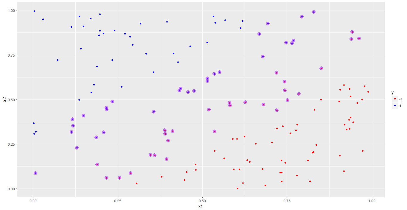
ggplot() を使って訓練データをプロットする。

# Visualize training data, distinguish classes using color
p <- ggplot(data = trainset, aes(x = x1, y = x2, color = y)) +
     geom_point() +
     scale_color_manual(values = c("red", "blue"))
# Render plot
p

svm_model の index を使ってサポートベクターを特定する。

# Identify support vectors
df_sv <- trainset[svm_model$index, ]
# Mark out support vectors in plot
p <- p + geom_point(data = df_sv,
                    aes(x = x1, y = x2),
                    color = "purple",
                    size = 4, alpha = 0.5)
# Display plot
p

第2章2節 - 線形分離可能データ、デフォルトコスト線形カーネル、サポートベクター付き

境界の傾きと切片を求める:

svm_model の coefs と SV から重みベクトル w を構築する。

# Build weight vector
w <- t(svm_model$coefs) %*% svm_model$SV

傾き =-w[1] / w[2]

# Calculate slope and save it to a variable
slope_1 <- -w[1] / w[2]

切片 = svm_model$rho / w[2]

# Calculate intercept and save it to a variable
intercept_1 <- svm_model$rho / w[2]

前のスライドで算出した傾きと切片を使って決定境界を追加する。
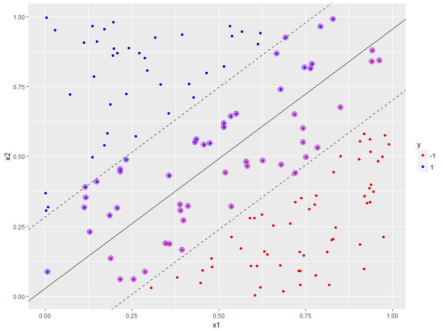
geom_abline() を使って決定境界をプロットに追加する。

# Plot decision boundary based on calculated slope and intercept
p <- p + geom_abline(slope = slope_1,
                     intercept = intercept_1)

マージンは決定境界に平行で、両側に 1 / w[2] だけオフセットされる。

# Add margins to plot
p <- p + 
    geom_abline(slope = slope_1,
                intercept = intercept_1 - 1 / w[2],
                linetype = "dashed") + 
    geom_abline(slope = slope_1,
                intercept = intercept_1 + 1 / w[2],
                linetype = "dashed")
# Display plot
p

第2章2節 - 線形分離可能データ、デフォルトコスト線形カーネル、サポートベクター・決定境界・マージン境界付き

ソフトマージン分類器

境界の位置・形状に不確実性を許容する
- 完全に線形にはならない
- 通常は未知
決定境界が線形のため、マージンを縮小できる

svm の plot() 関数による決定境界の可視化

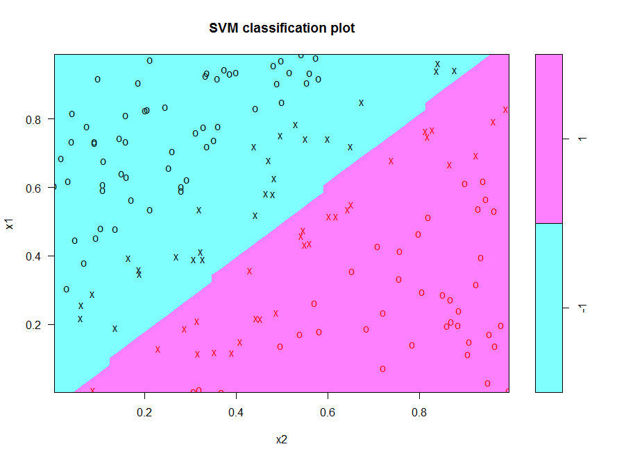
e1071 の plot() 関数を使うと、決定境界を簡単にプロットできます。

# Visualize decision boundary using built in plot function
plot(x = svm_model,
     data = trainset)

第2章2節 - 線形分離可能データ、デフォルトコスト線形カーネル、svm.plotによるプロット

練習しましょう！

Rで学ぶSupport Vector Machines