データの変動性の再現

R による欠損データの補完処理

Michal Oleszak

Machine Learning Engineer

補完データの変動性

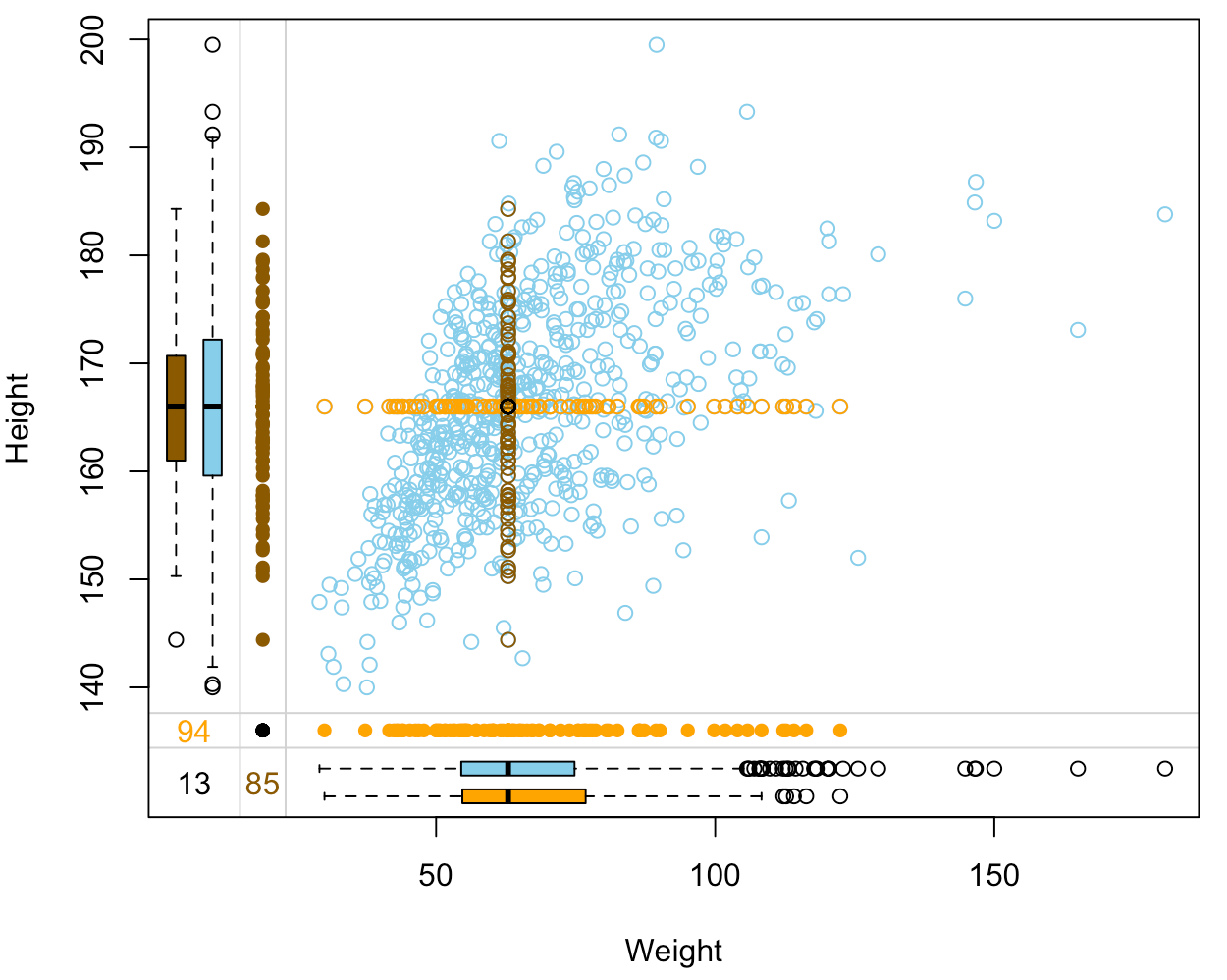
「Height」と「Weight」の散布図(マージンプロット)。いずれかの変数で補完された値が別の色でハイライトされている。

  • 補完データに変動性がない。
  • 補完は観測データの変動性を再現することが望ましい。
  • モデルベース補完では、予測変数が同じなら補完値も同じになる。
  • 解決策:条件付き分布からのサンプリング。
R による欠損データの補完処理

予測とは何か

多くの統計モデルは、応答変数の条件付き分布を推定する:

$p(y|X)$

単一の予測を行うには、条件付き分布を要約する:

  • 線形回帰:条件付き分布の期待値。
  • ロジスティック回帰:最も確率の高いクラス。

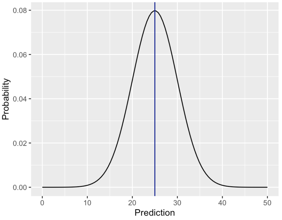
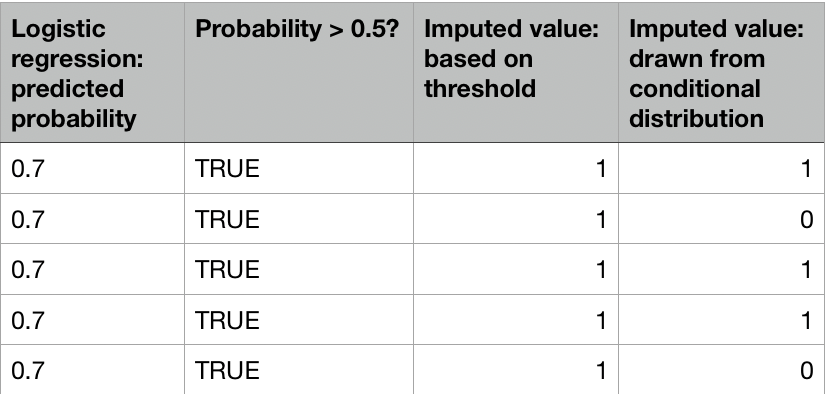
変動性を高めるには、これらの分布からサンプリングする。

R による欠損データの補完処理

条件付き分布からのサンプリング

正規分布の確率密度関数を示すグラフ。平均値25がハイライトされている。

R による欠損データの補完処理

条件付き分布からのサンプリング

4列のテーブル:ロジスティック回帰の予測確率(全行0.7)、確率が0.5超かどうか(全行TRUE)、閾値に基づく補完値(全行1)、条件付き分布から抽出した補完値(大半は1、一部は0)。

R による欠損データの補完処理

ロジスティック回帰による補完

タスク:ロジスティック回帰でnhanesデータのPhysActiveを補完する。

nhanes_imp <- hotdeck(nhanes)
missing_physactive <- is.na(nhanes$PhysActive)
R による欠損データの補完処理

ロジスティック回帰による補完

タスク:ロジスティック回帰でnhanesデータのPhysActiveを補完する。

nhanes_imp <- hotdeck(nhanes)
missing_physactive <- is.na(nhanes$PhysActive)
logreg_model <- glm(PhysActive ~ Age + Weight + Pulse, 
                    data = nhanes_imp, family = binomial)
R による欠損データの補完処理

ロジスティック回帰による補完

タスク:ロジスティック回帰でnhanesデータのPhysActiveを補完する。

nhanes_imp <- hotdeck(nhanes)
missing_physactive <- is.na(nhanes$PhysActive)
logreg_model <- glm(PhysActive ~ Age + Weight + Pulse, 
                    data = nhanes_imp, family = binomial)
preds <- predict(logreg_model, type = "response")
R による欠損データの補完処理

ロジスティック回帰による補完

タスク:ロジスティック回帰でnhanesデータのPhysActiveを補完する。

nhanes_imp <- hotdeck(nhanes)
missing_physactive <- is.na(nhanes$PhysActive)
logreg_model <- glm(PhysActive ~ Age + Weight + Pulse, 
                    data = nhanes_imp, family = binomial)
preds <- predict(logreg_model, type = "response")
preds <- ifelse(preds >= 0.5, 1, 0)
R による欠損データの補完処理

ロジスティック回帰による補完

タスク:ロジスティック回帰でnhanesデータのPhysActiveを補完する。

nhanes_imp <- hotdeck(nhanes)
missing_physactive <- is.na(nhanes$PhysActive)
logreg_model <- glm(PhysActive ~ Age + Weight + Pulse, 
                    data = nhanes_imp, family = binomial)
preds <- predict(logreg_model, type = "response")
preds <- ifelse(preds >= 0.5, 1, 0)
nhanes_imp[missing_physactive, "PhysActive"] <- preds[missing_physactive]
R による欠損データの補完処理

ロジスティック回帰による補完

補完データの変動性:

table(preds[missing_physactive])
 1 
26

観測済みPhysActiveデータの変動性:

table(nhanes$PhysActive)
  0   1 
181 610
R による欠損データの補完処理

クラス確率からのサンプリング

nhanes_imp <- hotdeck(nhanes)
missing_physactive <- is.na(nhanes$PhysActive)
logreg_model <- glm(PhysActive ~ Age + Weight + Pulse, 
                    data = nhanes_imp, family = binomial)
preds <- predict(logreg_model, type = "response")
preds <- ifelse(preds >= 0.5, 1, 0)
nhanes_imp[missing_physactive, "PhysActive"] <- preds[missing_physactive]
R による欠損データの補完処理

クラス確率からのサンプリング

nhanes_imp <- hotdeck(nhanes)
missing_physactive <- is.na(nhanes$PhysActive)
logreg_model <- glm(PhysActive ~ Age + Weight + Pulse, 
                    data = nhanes_imp, family = binomial)
preds <- predict(logreg_model, type = "response")

nhanes_imp[missing_physactive, "PhysActive"] <- preds[missing_physactive]
R による欠損データの補完処理

クラス確率からのサンプリング

nhanes_imp <- hotdeck(nhanes)
missing_physactive <- is.na(nhanes$PhysActive)
logreg_model <- glm(PhysActive ~ Age + Weight + Pulse, 
                    data = nhanes_imp, family = binomial)
preds <- predict(logreg_model, type = "response")
preds <- rbinom(length(preds), size = 1, prob = preds)
nhanes_imp[missing_physactive, "PhysActive"] <- preds[missing_physactive]
R による欠損データの補完処理

クラス確率からのサンプリング

補完データの変動性:

table(preds[missing_physactive])
0  1 
5 21

観測済みPhysActiveデータの変動性:

table(nhanes$PhysActive)
  0   1 
181 610
R による欠損データの補完処理

データの変動性の再現を練習しましょう!

R による欠損データの補完処理

Preparing Video For Download...