Rによる多変量確率分布
Surajit Ray
Professor, University of Glasgow
summary(cars.pca)
Importance of components:
                       Comp.1 Comp.2 Comp.3 Comp.4 Comp.5 Comp.6 Comp.7 Comp.8  Comp.9
Standard deviation      2.378  1.443  0.710 0.5148 0.4280 0.3518 0.3241 0.2419 0.14896
Proportion of Variance  0.628  0.231  0.056 0.0294 0.0204 0.0138 0.0117 0.0065 0.00247
Cumulative Proportion   0.628  0.860  0.916 0.9453 0.9656 0.9794 0.9910 0.9975 1.00000
方法1
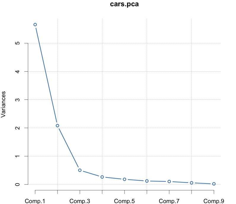
説明された変動の割合
screeplot(cars.pca, type = "lines")
選択の基準
方法2
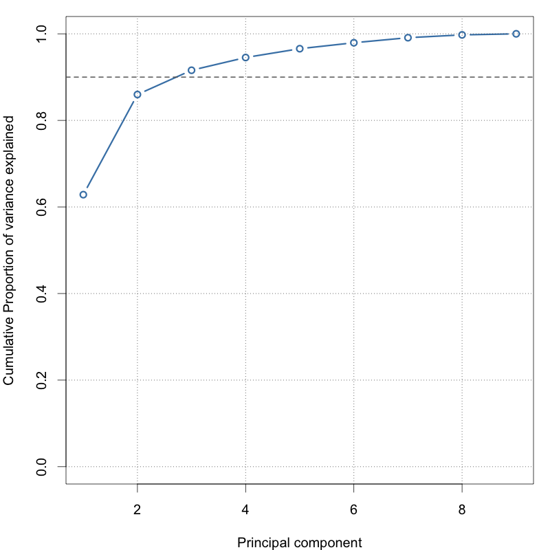
累積割合
# Variance explained
pc.var <- cars.pca$sdev^2

# Proportion of variation
pc.pvar <- pc.var / sum(pc.var)

# Cumulative proportion
plot(cumsum(pc.pvar), type = 'b')
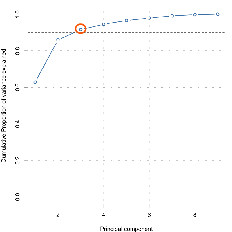
abline(h = 0.9, lty = 2)
3つのPCで変動の90%を説明