R によるカテゴリカルデータの推測
Andrew Bray
Assistant Professor of Statistics at Reed College
SE
0.009998905
SE_small_n
0.03809731
SE_low_p
0.00547912
標準誤差が大きくなる条件
n
p
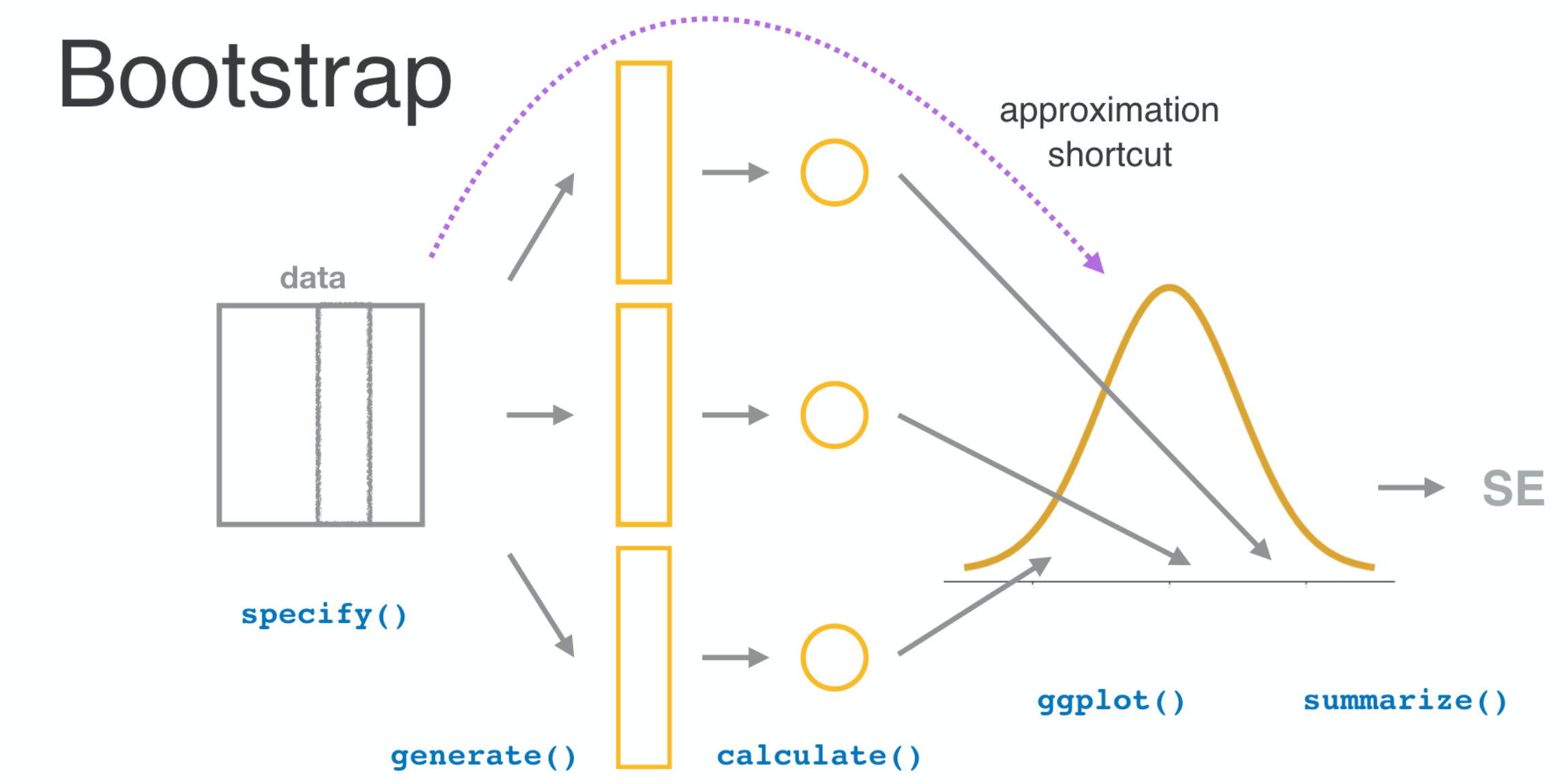
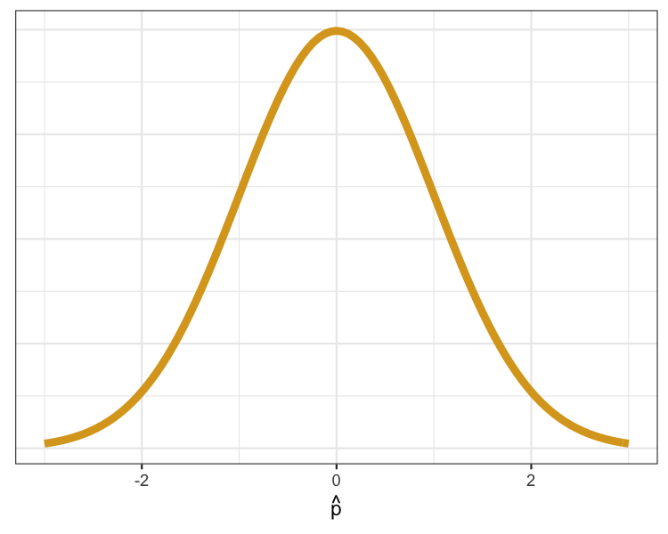
いわゆる「ベルカーブ」。
【もし】
【なら】
$$\sqrt{\frac{ \hat{p} \times (1 - \hat{p})}{n}}$$
「観測が独立」かはどう確認しますか?
「n が大きい」とは?
p_hat <- gss2016 %>%
  summarize(mean(happy == "HAPPY")) %>%
  pull()
n <- nrow(gss2016)
c(n * p_hat, n * (1 - p_hat))
116 35
SE_approx <- sqrt(p_hat * (1 - p_hat) / n)
SE_approx
0.03418468
boot <- gss2016 %>%
  specify(response = happy, success = "HAPPY") %>%
  generate(reps = 500, type = "bootstrap") %>%
  calculate(stat = "prop")
SE_boot <- boot %>%
  summarize(sd(stat)) %>%
  pull()
SE_boot
0.03176741
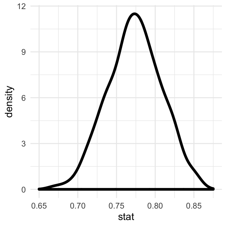
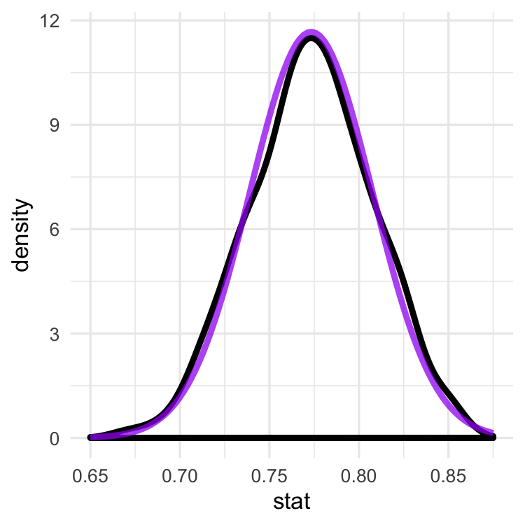
ggplot(boot, aes(x = stat)) +
  geom_density()
ggplot(boot, aes(x = stat)) +
  geom_density() +
  stat_function(fun = dnorm,
                color = "purple",
                args =
                  list(mean = p_hat,
                       sd = SE_approx))