信頼区間の解釈

R によるカテゴリカルデータの推測

Andrew Bray

Assistant Professor of Statistics at Reed College

信頼区間

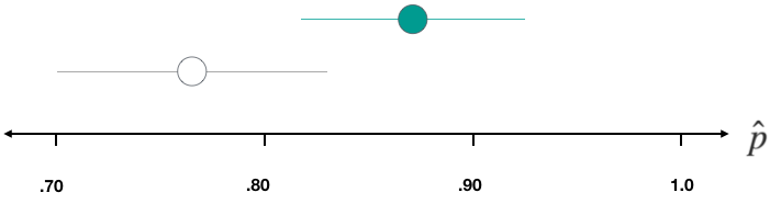
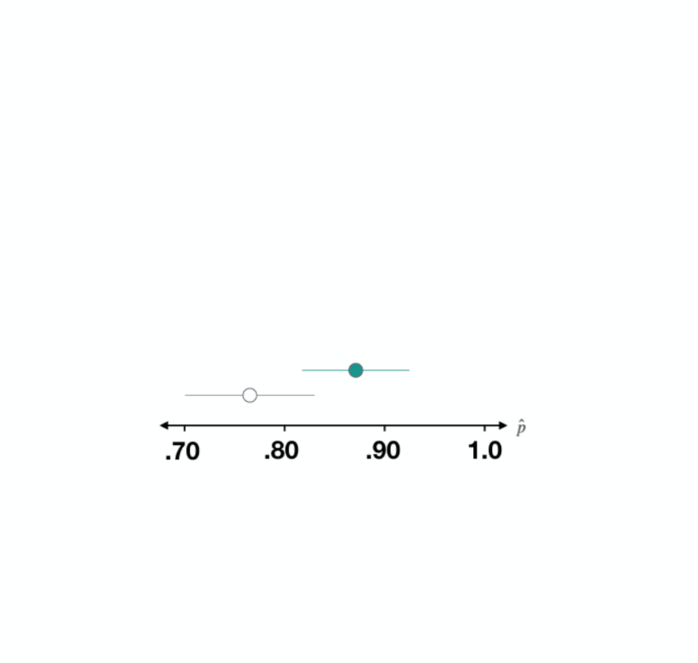
結論：幸せなアメリカ人の真の割合は 0.705〜0.841 の間にあります。

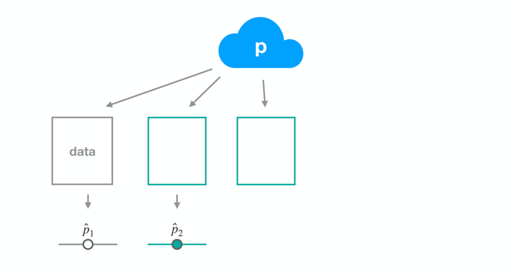
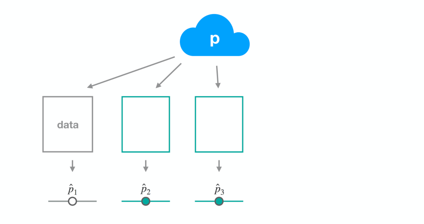
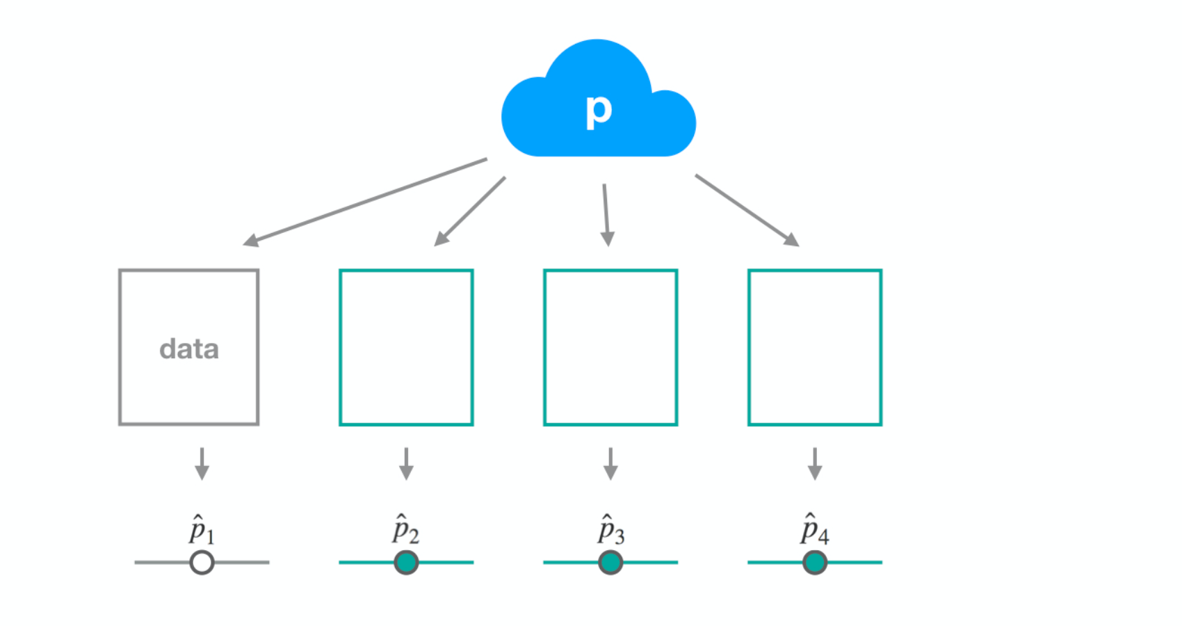
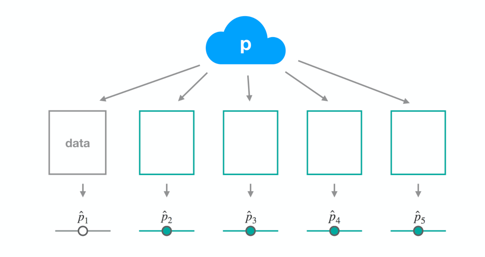
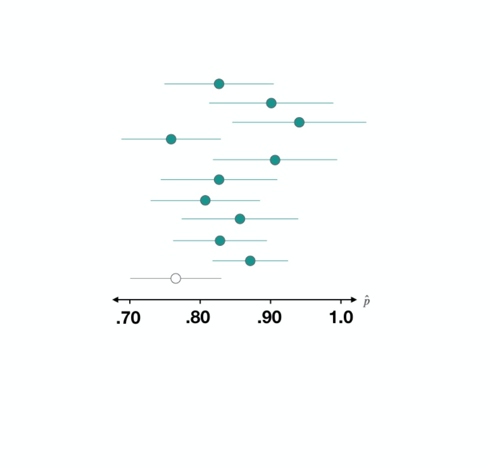
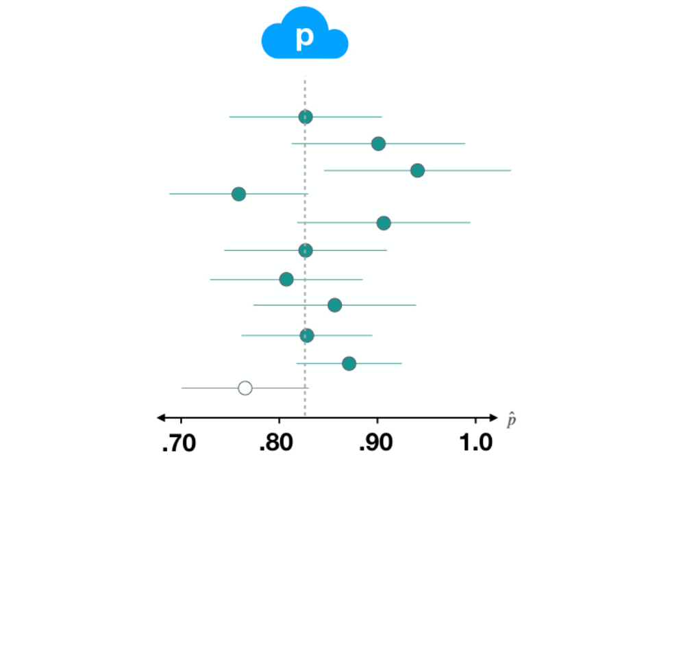
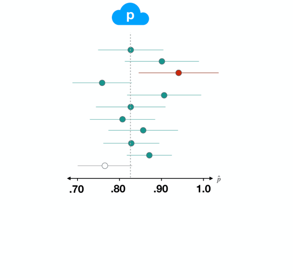
「自信がある」とは何を意味しますか。

データセット 1

ds1 <- filter(gss, year == 2016)

p_hat <- ds1 %>%
  summarize(mean(happy == "HAPPY")) %>% 
  pull()

SE <- ds1 %>%
  specify(response = happy, 
          success = "HAPPY") %>%
  generate(reps = 500, 
           type = "bootstrap") %>%
  calculate(stat = "prop") %>%
  summarize(sd(stat)) %>% 
  pull()

c(p_hat - 2 * SE, p_hat + 2 * SE)

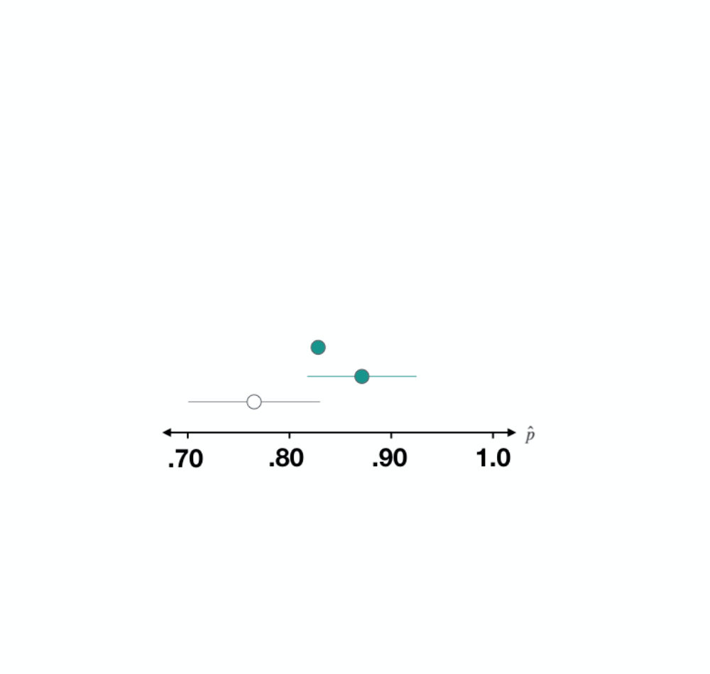
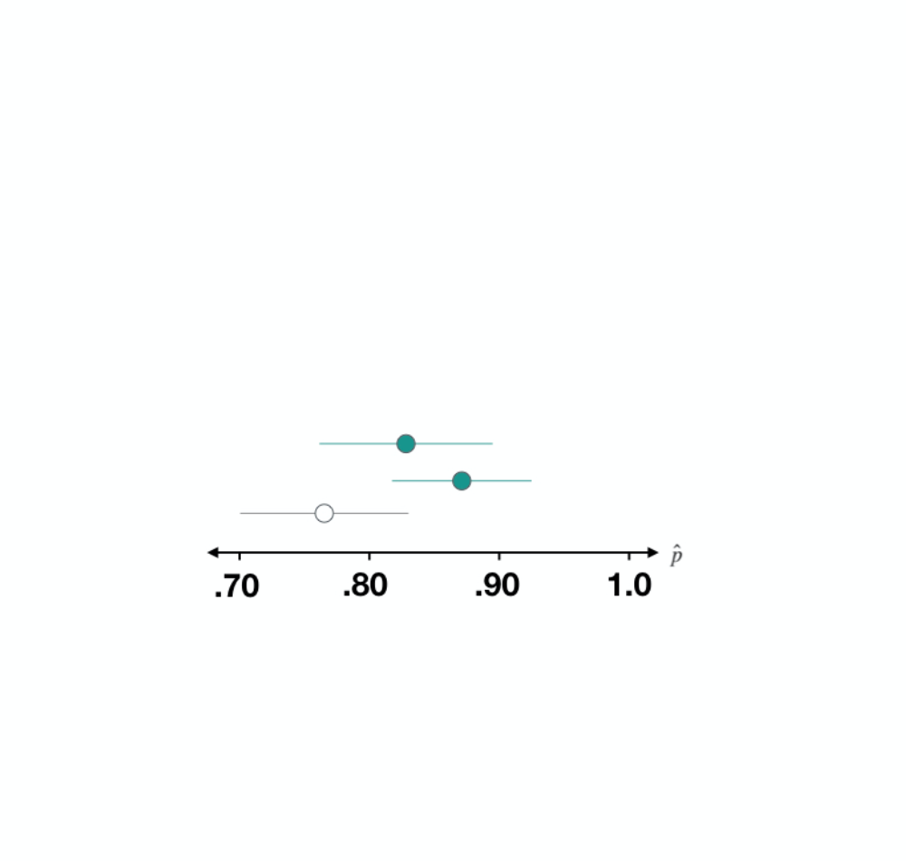
0.7073114 0.8393553

confidence-interval

データセット 2

ds2 <- filter(gss, year == 2014)

p_hat <- ds1 %>%
  summarize(mean(happy == "HAPPY")) %>% 
  pull()

SE <- ds1 %>%
  specify(response = happy, 
          success = "HAPPY") %>%
  generate(reps = 500, 
           type = "bootstrap") %>%
  calculate(stat = "prop") %>%
  summarize(sd(stat)) %>% 
  pull()

c(p_hat - 2 * SE, p_hat + 2 * SE)

0.8348831 0.9384503

Screenshot 2019-02-21 18.05.03.png

データセット 3

ds3 <- filter(gss, year == 2012)

p_hat <- ds1 %>%
  summarize(mean(happy == "HAPPY")) %>% 
  pull()

SE <- ds1 %>%
  specify(response = happy, 
          success = "HAPPY") %>%
  generate(reps = 500, 
           type = "bootstrap") %>%
  calculate(stat = "prop") %>%
  summarize(sd(stat)) %>% 
  pull()

c(p_hat - 2 * SE, p_hat + 2 * SE)

0.7626359 0.8906974

データセット 3

ds3 <- filter(gss, year == 2012)
p_hat <- ds3 %>%
  summarize(mean(happy == "HAPPY")) %>%
  pull()
SE <- ds3 %>%
  specify(response = happy, 
          success = "HAPPY") %>%
  generate(reps = 500, 
           type = "bootstrap") %>%
  calculate(stat = "prop") %>%
  summarize(sd(stat)) %>%
  pull()

c(p_hat - 2 * SE, p_hat + 2 * SE)

0.7626359 0.8906974

データセット 3

ds3 <- filter(gss, year == 2012)
p_hat <- ds3 %>%
  summarize(mean(happy == "HAPPY")) %>%
  pull()
SE <- ds3 %>%
  specify(response = happy, 
          success = "HAPPY") %>%
  generate(reps = 500, 
           type = "bootstrap") %>%
  calculate(stat = "prop") %>%
  summarize(sd(stat)) %>%
  pull()

c(p_hat - 2 * SE, p_hat + 2 * SE)

0.7626359 0.8906974

データセット 3

ds3 <- filter(gss, year == 2012)
p_hat <- ds3 %>%
  summarize(mean(happy == "HAPPY")) %>%
  pull()
SE <- ds3 %>%
  specify(response = happy, 
          success = "HAPPY") %>%
  generate(reps = 500, 
           type = "bootstrap") %>%
  calculate(stat = "prop") %>%
  summarize(sd(stat)) %>%
  pull()

c(p_hat - 2 * SE, p_hat + 2 * SE)

0.7626359 0.8906974

データセット 3

ds3 <- filter(gss, year == 2012)
p_hat <- ds3 %>%
  summarize(mean(happy == "HAPPY")) %>%
  pull()
SE <- ds3 %>%
  specify(response = happy, 
          success = "HAPPY") %>%
  generate(reps = 500, 
           type = "bootstrap") %>%
  calculate(stat = "prop") %>%
  summarize(sd(stat)) %>%
  pull()

c(p_hat - 2 * SE, p_hat + 2 * SE)

0.7626359 0.8906974

データセット 3

ds3 <- filter(gss, year == 2012)
p_hat <- ds3 %>%
  summarize(mean(happy == "HAPPY")) %>%
  pull()
SE <- ds3 %>%
  specify(response = happy, 
          success = "HAPPY") %>%
  generate(reps = 500, 
           type = "bootstrap") %>%
  calculate(stat = "prop") %>%
  summarize(sd(stat)) %>%
  pull()

c(p_hat - 2 * SE, p_hat + 2 * SE)

0.7626359 0.8906974

信頼区間

解釈：「幸せなアメリカ人の真の割合は 0.705〜0.841 の間にあると95%確信しています。」

区間の幅に影響するもの

n
信頼水準
p

練習しましょう！

R によるカテゴリカルデータの推測