エンリッチメントの評価

Rで学ぶBioconductorによるChIP-seq

Peter Humburg

Statistician, Macquarie University

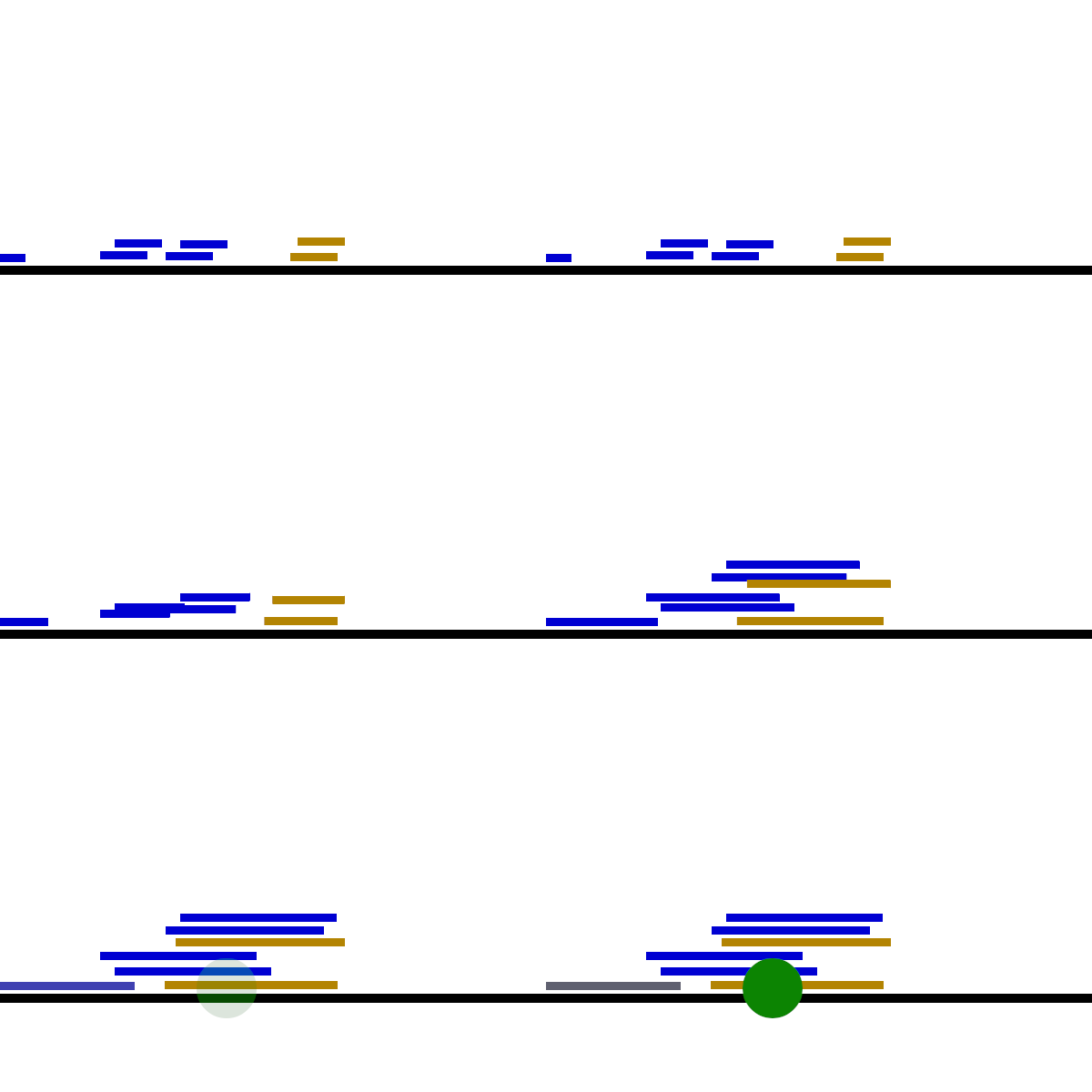
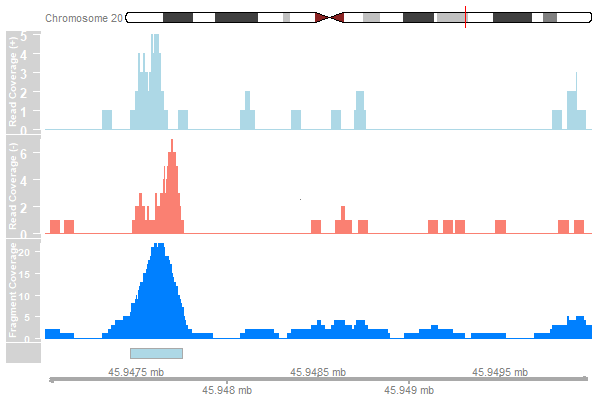
リードの伸長

データの読み込み:

reads <- readGAlignments(bam)
reads_gr <- granges(reads[[1]])

平均フラグメント長の取得:

frag_length <- fragmentlength(qc_report)["GSM1598218"]

リードを伸長してカバレッジを計算:

reads_ext <- resize(reads_gr, width=frag_length)
cover_ext <- coverage(reads_ext)

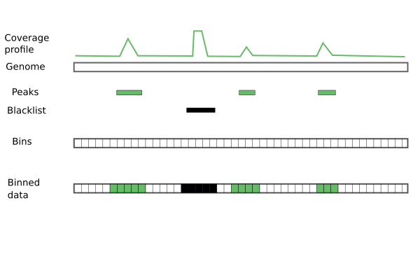
ピークのカバレッジ

ゲノム全体に200 bpのビンを作成します。

bins <- tileGenome(seqinfo(reads), tilewidth=200, 
                   cut.last.tile.in.chrom=TRUE)

ピークと重なるビンをすべて検索します。

peak_bins_overlap <- findOverlaps(bins, peaks)
peak_bins <- bins[from(peak_bins_overlap), ]

各ピークビンに重なるリード数をカウントします。

peak_bins$score <- countOverlaps(peak_bins, reads)

ビン化カバレッジ関数

count_bins <- function(reads, target, bins){
  # Find all bins overlapping peaks
  overlap <- from(findOverlaps(bins, target))
  target_bins <- bins[overlap, ]

  # Count the number of reads overlapping each peak bin
  target_bins$score <- countOverlaps(target_bins, reads)
  target_bins
}

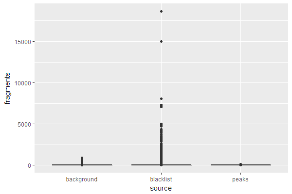
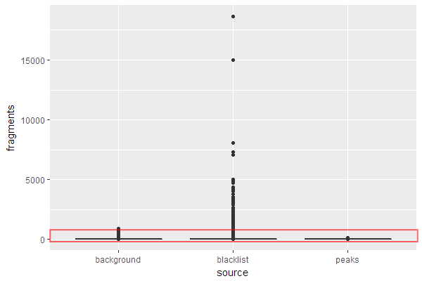
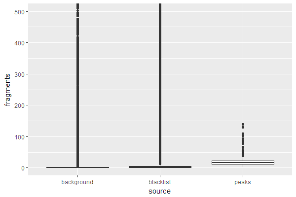
ブラックリスト領域のカバレッジ

peak_bins <- count_bins(reads_ext, peaks, bins)
bl_bins <- count_bins(reads_ext, blacklist.hg19, bins)

バックグラウンドカバレッジ

既に処理済みのビンをすべて除外します。

bkg_bins <- subset(bins, !bins %in% peak_bins & !bins %in% bl_bins)

残りの各ビンに重なるリード数をカウントします。

bkg_bins$score <- countOverlaps(bkg_bins, reads_ext)

では、練習しましょう！

Rで学ぶBioconductorによるChIP-seq