ピークの詳細分析
Rで学ぶBioconductorによるChIP-seq

Peter Humburg
Statistician, Macquarie University
Gviz の使用
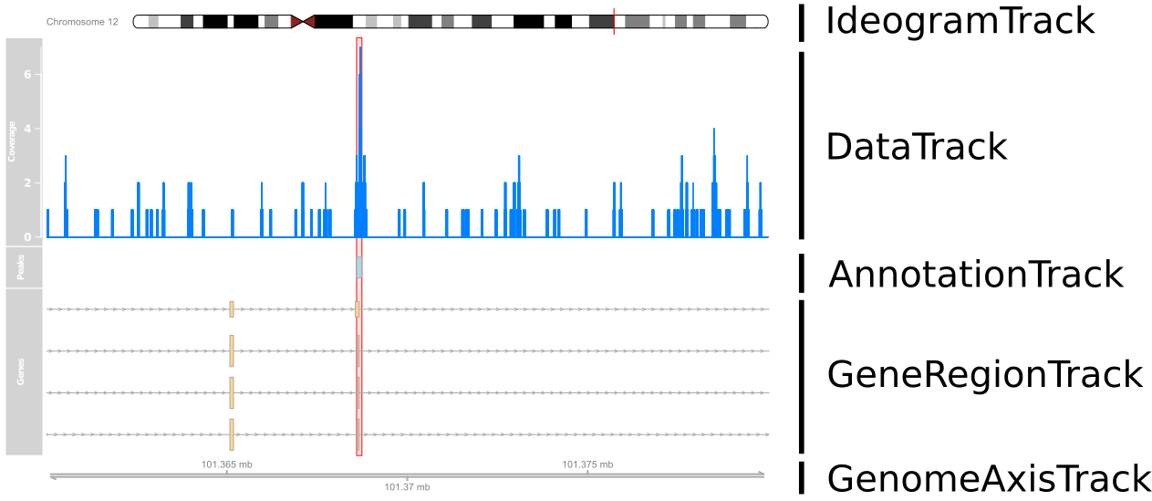
何をプロットしているか?
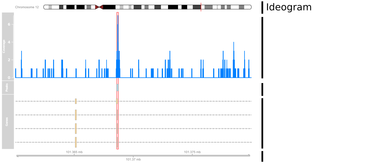
何をプロットしているか?
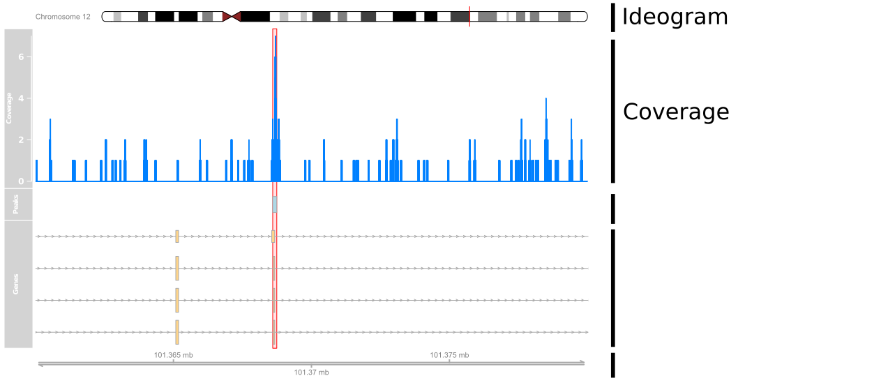
何をプロットしているか?
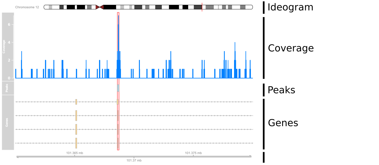
何をプロットしているか?
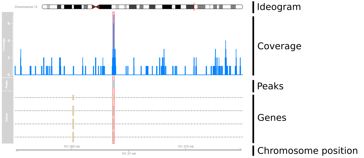
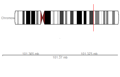
座標の設定
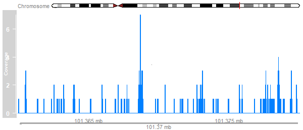
データの追加
cover_track <- DataTrack(cover_ranges,window=100000,type='h',name="Coverage")
plotTracks(list(ideogram, cover_track, axis), from=101360000, to=101380000)
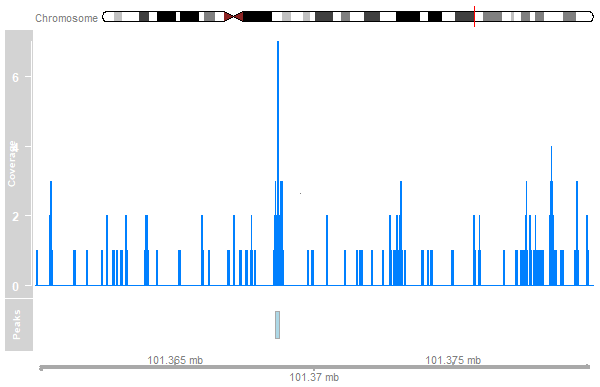
アノテーションの追加
peak_track <- AnnotationTrack(peaks, name="Peaks")
plotTracks(list(ideogram, cover_track, peak_track, axis),
           from=101360000, to=101380000)
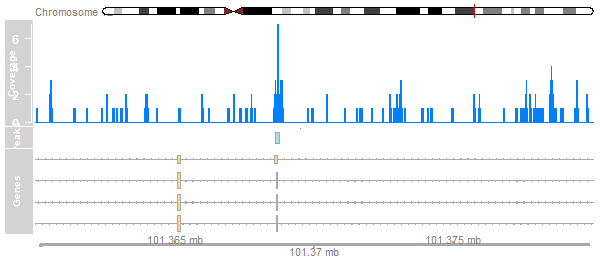
遺伝子アノテーション
library(TxDb.Hsapiens.UCSC.hg19.knownGene)tx <- GeneRegionTrack(TxDb.Hsapiens.UCSC.hg19.knownGene, chromosome="chr12", start=101360000, end=101380000, name="Genes") plotTracks(list(ideogram, cover_track, peak_track, tx, axis), from=101360000, to=101380000)