事前分布

rstanarm で学ぶベイズ回帰モデリング

Jake Thompson

Psychometrician, ATLAS, University of Kansas

事前分布とは？

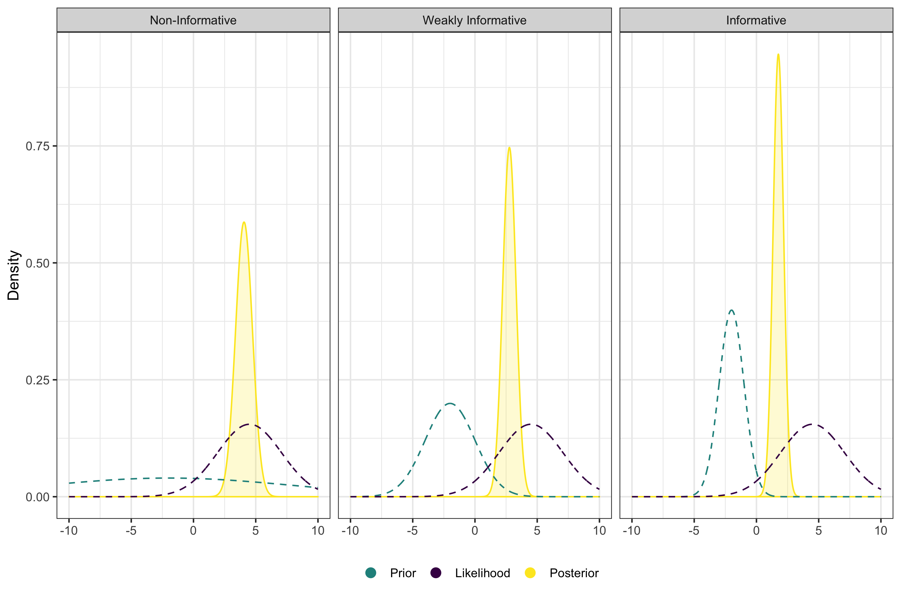
モデルに組み込む事前情報
尤度 + 事前分布 = 事後分布

rstanarm における事前分布

stan_model <- stan_glm(kid_score ~ mom_iq, data = kidiq)
prior_summary(stan_model)

Priors for model 'stan_model' 
 ------
Intercept (after predictors centered)
 ~ normal(location = 0, scale = 10)
     **adjusted scale = 204.11
Coefficients
 ~ normal(location = 0, scale = 2.5)
     **adjusted scale = 3.40
Auxiliary (sigma)
 ~ exponential(rate = 1)
     **adjusted scale = 20.41 (adjusted rate = 1/adjusted scale)
 ------
See help('prior_summary.stanreg') for more details

調整済みスケールの計算

切片：10 * sd(y)
係数：(2.5 / sd(x)) * sd(y)

prior_summary(stan_model)

Priors for model 'stan_model' 
 ------
Intercept (after predictors centered)
 ~ normal(location = 0, scale = 10)
     **adjusted scale = 204.11

Coefficients
 ~ normal(location = 0, scale = 2.5)
     **adjusted scale = 3.40

10 * sd(kidiq$kid_score)

204.1069

(2.5 / sd(kidiq$mom_iq)) * sd(kidiq$kid_score)

3.401781

no_scale <- stan_glm(kid_score ~ mom_iq, data = kidiq,
  prior_intercept = normal(autoscale = FALSE),
  prior = normal(autoscale = FALSE),
  prior_aux = exponential(autoscale = FALSE))
prior_summary(no_scale)

Priors for model 'no_scale' 
 ------
Intercept (after predictors centered)
 ~ normal(location = 0, scale = 10)

Coefficients
 ~ normal(location = 0, scale = 2.5)

Auxiliary (sigma)
 ~ exponential(rate = 1)
 ------
See help('prior_summary.stanreg') for more details

練習しましょう！

rstanarm で学ぶベイズ回帰モデリング