summary(stan_model)
Model Info:

 function:     stan_glm
 family:       gaussian [identity]
 formula:      kid_score ~ mom_iq
 algorithm:    sampling
 priors:       see help('prior_summary')
 sample:       1500 (posterior sample size)
 observations: 434
 predictors:   2

Estimates:
                mean    sd      2.5%    25%     50%     75%     97.5%
(Intercept)      25.8     6.0    14.1    21.7    25.6    29.9    37.5
mom_iq            0.6     0.1     0.5     0.6     0.6     0.7     0.7
sigma            18.3     0.6    17.2    17.9    18.3    18.7    19.6
mean_PPD         86.9     1.3    84.5    86.0    86.9    87.7    89.2
log-posterior -1885.4     1.2 -1888.4 -1885.9 -1885.1 -1884.5 -1884.0

Diagnostics:
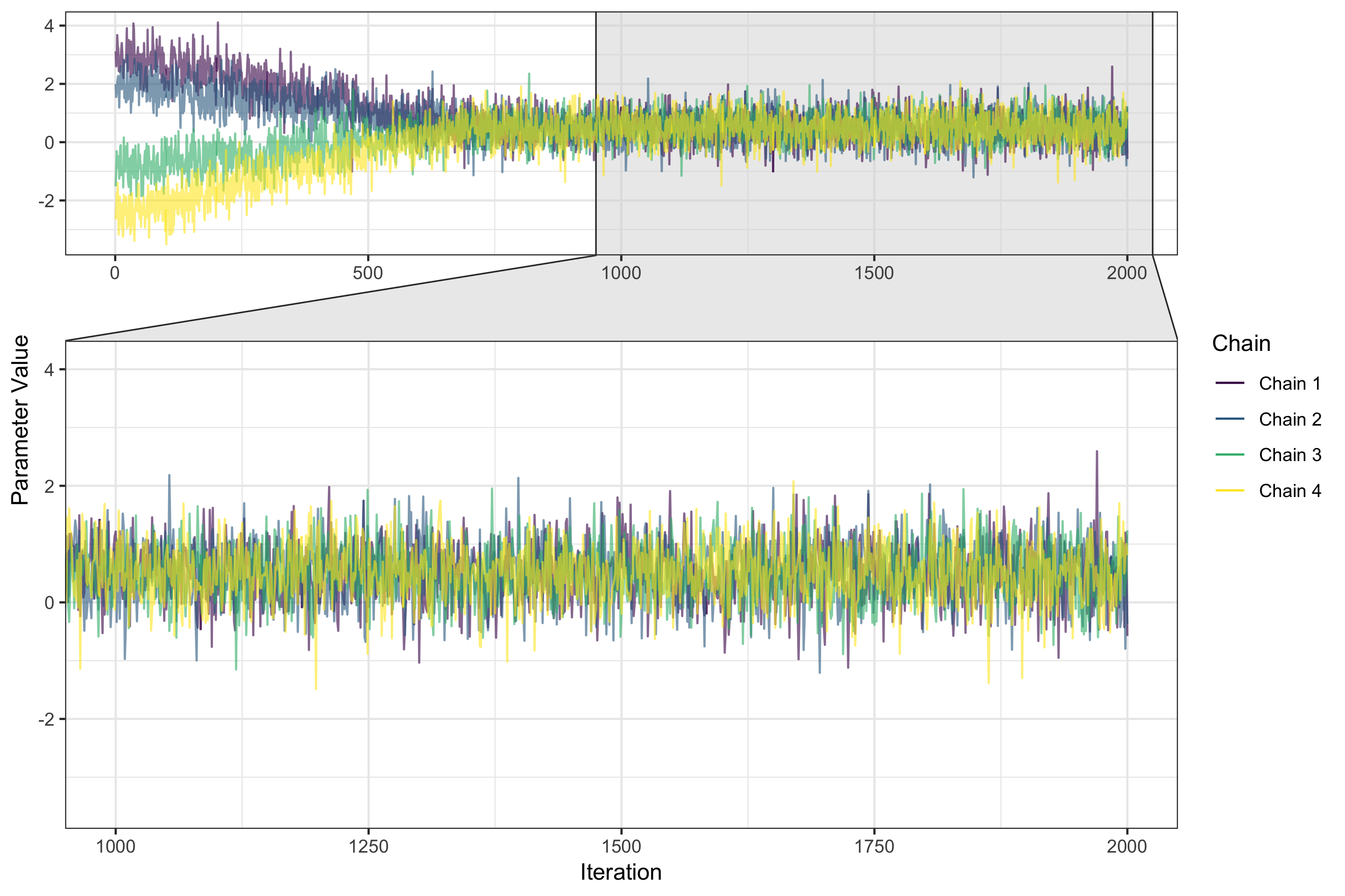
              mcse Rhat n_eff
(Intercept)   0.2  1.0  1500
mom_iq        0.0  1.0  1500
sigma         0.0  1.0  1500
mean_PPD      0.0  1.0  1500
log-posterior 0.0  1.0   619

For each parameter, mcse is Monte Carlo standard error, n_eff is a crude measure of effective sample size, and Rhat is the potential scale reduction factor on split chains (at convergence Rhat=1).