時間の特徴量

Rで学ぶ不正検知

Bart Baesens

Professor Data Science at KU Leuven

時間の分析

ある種のイベントは似た時刻に発生しやすい
例：顧客が似た時間帯に取引する
目的：時間情報を意味のある特徴量で捉える
時間の扱いは難しい
- 00:00 = 24:00
- 自然な順序がない（例：23:00 は 01:00 より小さいか大きいか？）

タイムスタンプの平均に算術平均は使わない！
- 例：01:00、02:00、21:00、22:00 に取引
- 算術平均は 11:30 だが、その近くで取引はない！

head(timestamps)

"20:27:28" "21:08:41" "01:30:16" "00:57:04" "23:12:14" "22:54:16"

デジタル時刻を時間の10進表記に変換

library(lubridate)
ts <- as.numeric(hms(timestamps)) / 3600

head(ts)

20.4577778 21.1447222  1.5044444  0.9511111 23.2038889 22.9044444

円形ヒストグラム

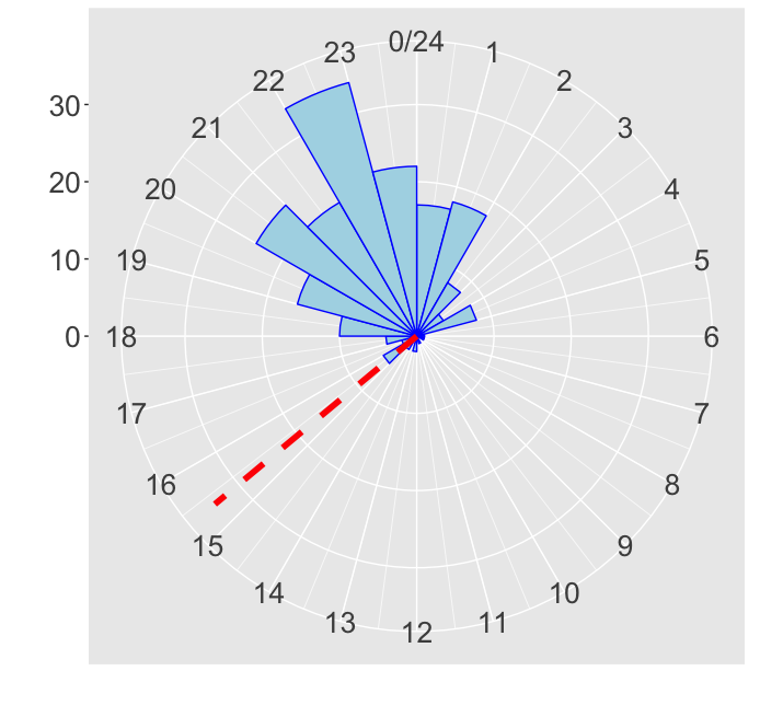
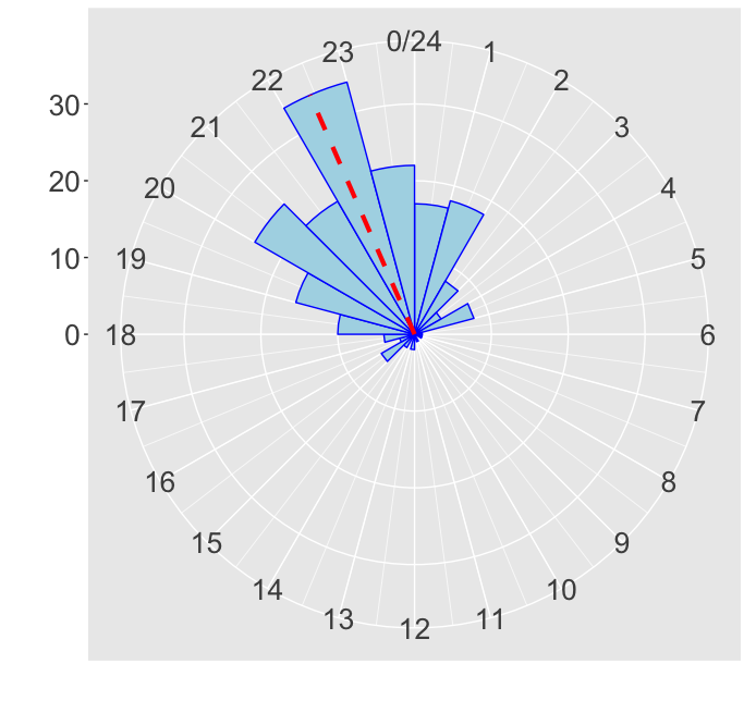
library(ggplot2)

clock <- ggplot(data.frame(ts), aes(x = ts)) +
    geom_histogram(breaks = seq(0, 24), colour = "blue", fill = "lightblue") +
    coord_polar()


arithmetic_mean <- mean(ts)

clock + geom_vline(xintercept = arithmetic_mean,
                     linetype = 2, color = "red", size = 2)

算術平均による円形ヒストグラム

誤った時計

von Mises 確率分布

時刻を周期変数として、von Mises 分布でモデル化（Correa Bahnsen ほか, 2016）
周期正規分布＝正規分布を円環に巻いたもの
タイムスタンプ集合 $D= $ {$t_1, t_2, \ldots, t_n$} の von Mises 分布

$$D\sim vonMises\left(\mu,\kappa\right)$$

$\mu$：周期平均（位置の指標）、分布は $\mu$ 付近に集中
$1/\kappa$：周期分散；$\kappa$ は集中度

パラメータ $\mu$ と $\kappa$ の推定

# 10進法のタイムスタンプを「circular」クラスに変換
library(circular)
ts <- circular(ts, units = "hours", template = "clock24")

head(ts)

Circular Data: 
[1] 20.457889 21.144607  1.504422  0.950982 23.203917  4.904397

estimates <- mle.vonmises(ts)
p_mean <- estimates$mu %% 24
concentration <- estimates$kappa

周期平均つきの円形ヒストグラム

正しい時計

信頼区間

新しい特徴量を抽出：取引時刻の信頼区間
$S= $ {$x_i^{time}|i=1,\ldots,n$} ：同一顧客の取引集合

(1) mle.vonmises() で $S$ に基づき $\mu(S)$ と $\kappa(S)$ を推定:

estimates <- mle.vonmises(ts)
p_mean <- estimates$mu %% 24
concentration <- estimates$kappa

(2) dvonmises() で各タイムスタンプの密度（=尤度）を計算:

densities <- dvonmises(ts, mu = p_mean, kappa = concentration)

特徴量抽出

二値特徴量：新規取引の時刻が信頼区間（CI）内に入る確率は $\alpha$（例: 0.90, 0.95）
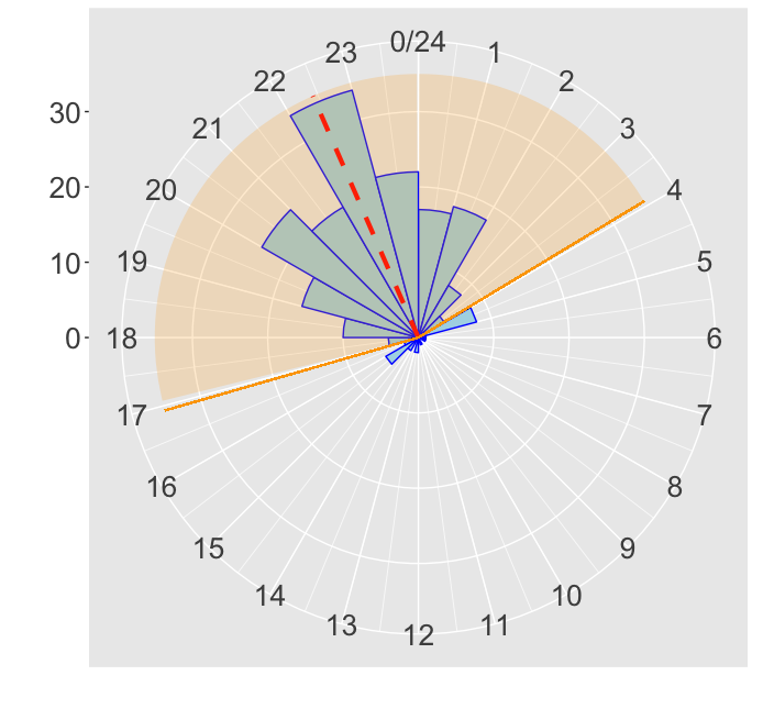
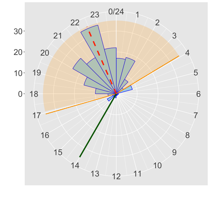
時刻がCI内なら TRUE、それ以外は FALSE
90% CI 内とは、密度がカットオフ値より大きい場合：

alpha <- 0.90
quantile <- qvonmises(p = (1 - alpha)/2, 
                        mu = p_mean,
                        kappa = concentration) %% 24
cutoff <- dvonmises(quantile,
                      mu = p_mean, kappa = concentration)

time_feature <- densities >= cutoff

信頼区間

信頼区間の時計

信頼区間

信頼区間の時計 2

例

$$ $$ 時間テーブル

移動ウィンドウでの信頼区間

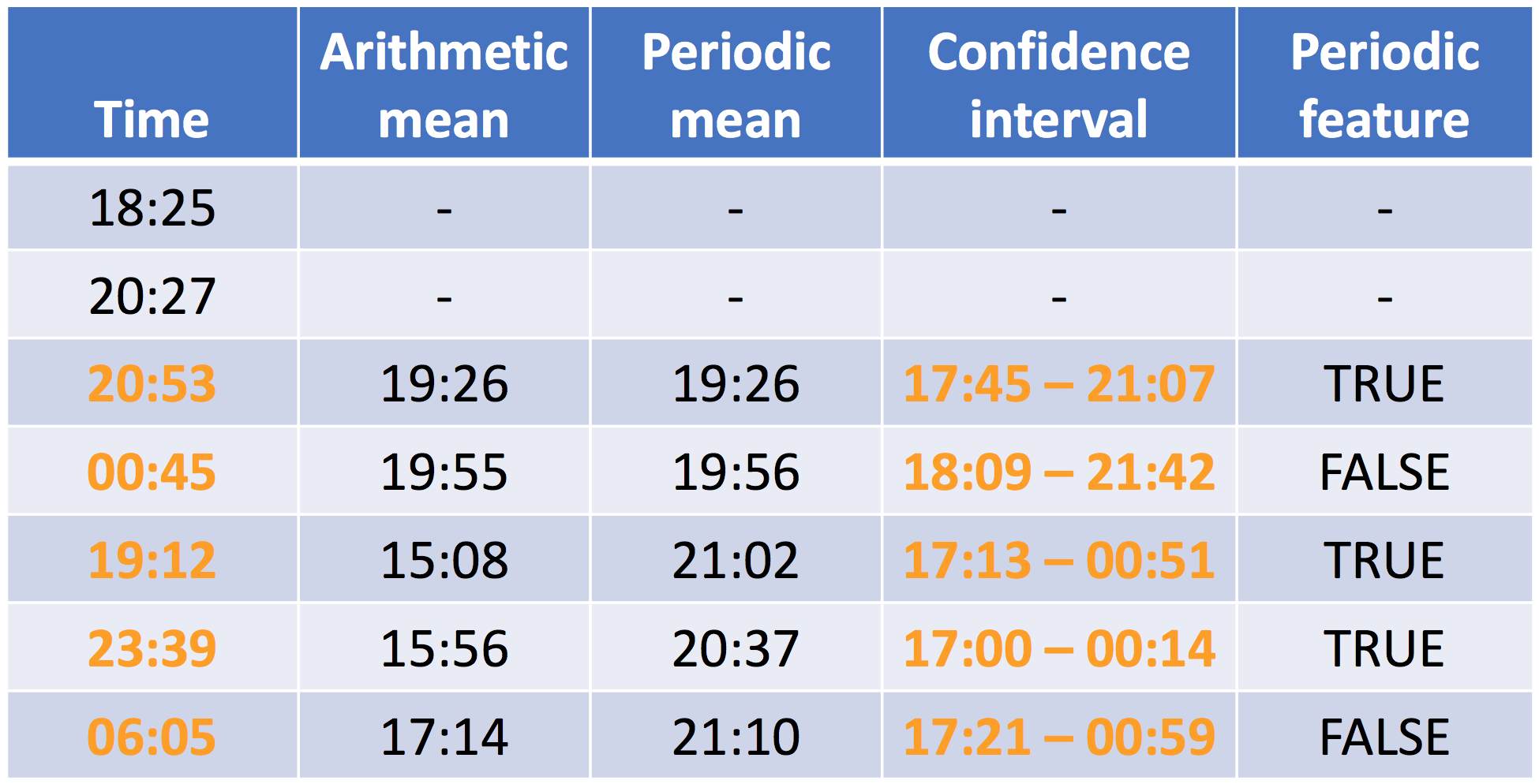
## ts には 18.42, 20.45, 20.88, 0.75, 19.20, 23.65, 6.08 のタイムスタンプが含まれる

time_feature = c(NA, NA)
for (i in 3:length(ts)) {
    ts_history <- ts[1:(i-1)] ## (1) 直前までの時刻

    estimates <- mle.vonmises(ts_history) ## (2) 過去データで mu と kappa を推定
    p_mean <- estimates$mu %% 24
    concentration <- estimates$kappa

    dens_i <- dvonmises(ts[i], mu = p_mean, kappa = concentration) ## (3) 現在の時刻の密度を算出

    alpha <- 0.90 ## (4) 信頼水準 90% のカットオフ超えか判定
    quantile <- qvonmises((1-alpha)/2, mu=p_mean, kappa=concentration) %% 24
    cutoff <- dvonmises(quantile, mu = p_mean, kappa = concentration)
    time_feature[i] <- dens_i >= cutoff
}

print(time_feature)

NA    NA  TRUE FALSE  TRUE  TRUE FALSE

Let's practice!

Rで学ぶ不正検知