ガウス分布

R で学ぶ Mixture Models

Victor Medina

Researcher at The University of Edinburgh

混合モデルと性別データセット

混合モデルのフィッティング用パッケージ

mixtools
- ポアソン分布は実装されていない。
bayesmix
- ベイズ推論はコースの範囲外。
EMCluster
- ガウス分布のみ対応。
flexmix
- 必要なすべての分布に対応し、より複雑なモデルにも柔軟に利用できる。

ガウス分布の性質

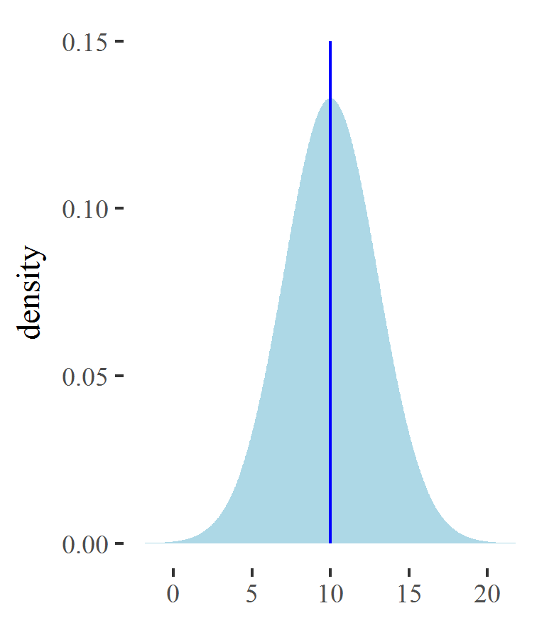
平均

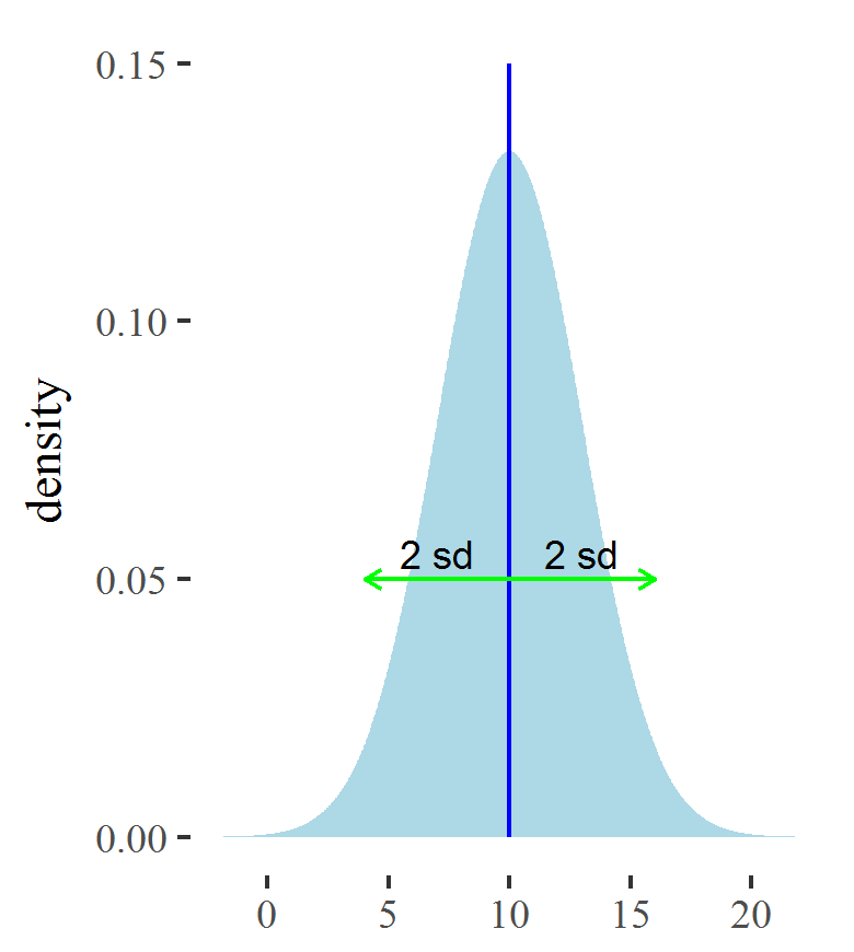
標準偏差

ガウス分布からのサンプリング

ガウス分布からサンプルを生成するには：

rnorm(n, mean, sd)

例：平均10、標準偏差5のガウス分布から100個の値を生成する

> population_sample <- rnorm(n = 100, mean = 10, sd = 5)
> head(population_sample)

[1]  6.248874  9.564190 16.006521  9.139647 10.114969 16.423538

平均の推定

平均と標準偏差は不明で、観測値のみ既知
- 観測値から推定する必要がある
平均の推定には標本平均を計算する

> mean_estimate <- mean(population_sample)

10.35759

sd の推定手順

$$value_i\rightarrow (. -mean\_estimate)\rightarrow (.)^2\rightarrow mean (.)\rightarrow \sqrt{(.)}$$

> population_sample %>%  
+   subtract(mean_estimate) %>%
+   raise_to_power(2) %>% mean() %>% sqrt()

5.318641

sd 関数の使用

> standard_deviation_estimate <- sd(population_sample)
> standard_deviation_estimate

5.345435

推定ガウス分布の可視化

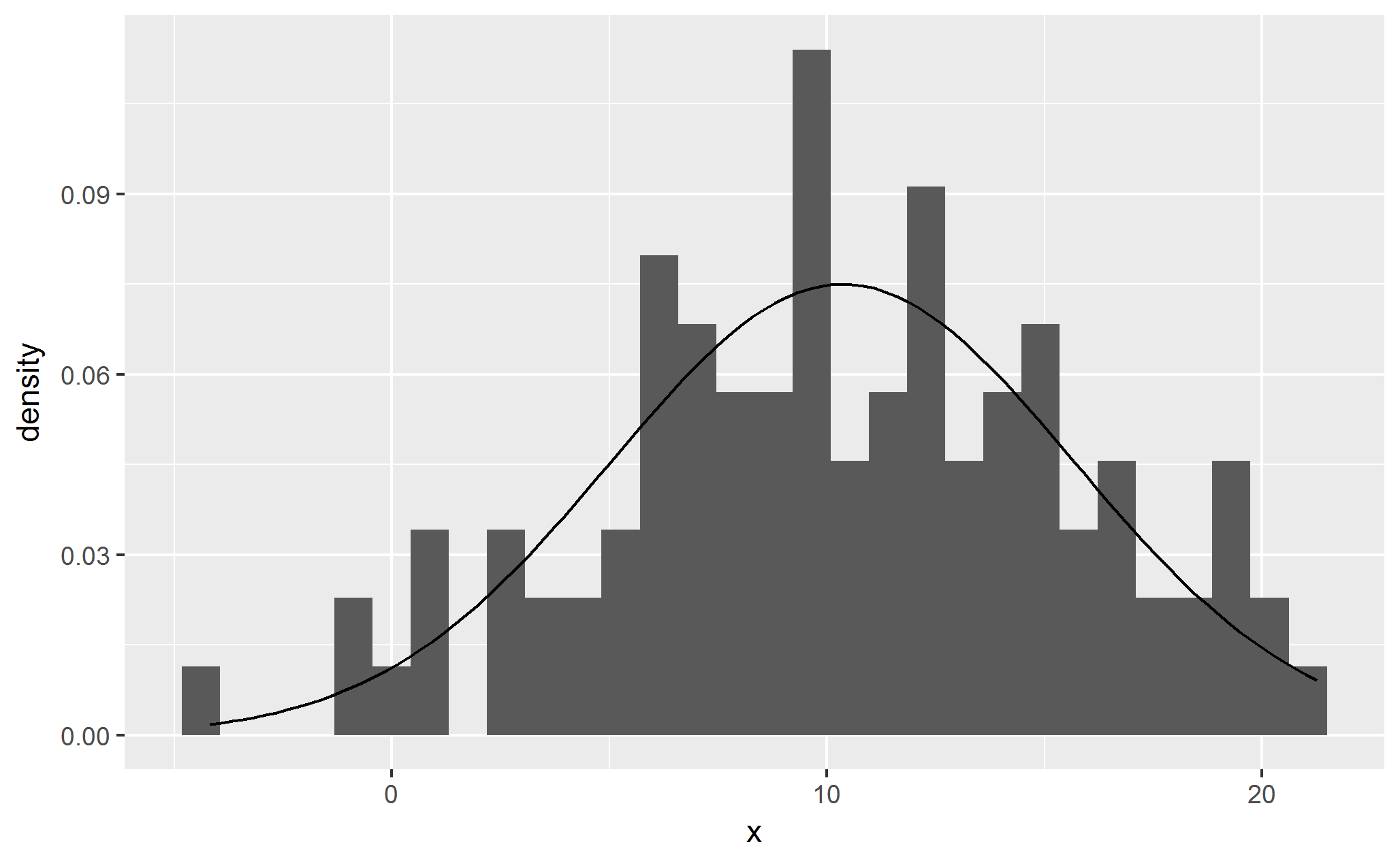
# Transform the sample into a data frame
population_sample <- data.frame(x = population_sample)

# Plot the histogram
ggplot(data = population_sample) + 
   geom_histogram(aes(x = x, y = ..density..)) +
   stat_function(geom = "line", 
                 fun = dnorm, 
                 args = list(mean = mean_estimate, 
                             sd = standard_deviation_estimate))

さあ、練習しましょう！

R で学ぶ Mixture Models