Why you need logistic regression

Nhập môn Hồi quy bằng R

Richie Cotton

Data Evangelist at DataCamp

Bank churn dataset

has_churned	time_since_first_purchase	time_since_last_purchase
0	0.3993247	-0.5158691
1	-0.4297957	0.6780654
0	3.7383122	0.4082544
0	0.6032289	-0.6990435
...	...	...
response	length of relationship	recency of activity

¹ https://www.rdocumentation.org/packages/bayesQR/topics/Churn

Churn vs. recency: a linear model

mdl_churn_vs_recency_lm <- lm(has_churned ~ time_since_last_purchase, data = churn)

Call:
lm(formula = has_churned ~ time_since_last_purchase, data = churn)

Coefficients:
             (Intercept)  time_since_last_purchase  
                 0.49078                   0.06378

coeffs <- coefficients(mdl_churn_vs_recency_lm)
intercept <- coeffs[1]
slope <- coeffs[2]

Visualizing the linear model

ggplot(
  churn, 
  aes(time_since_last_purchase, has_churned)
) +
  geom_point() +
  geom_abline(intercept = intercept, slope = slope)

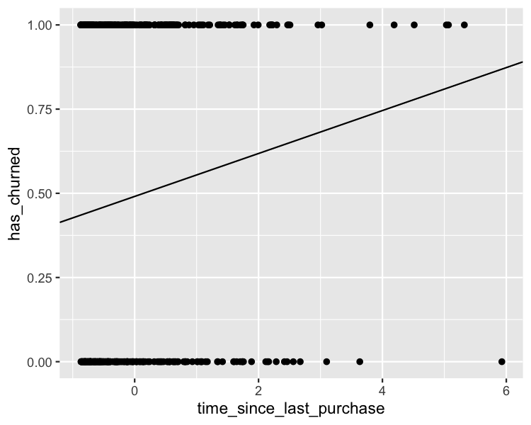
Predictions are probabilities of churn, not amounts of churn.

A scatter plot of whether or not the customer churned versus time since last purchase. All the points are at the line y equals 0 or y equals 1. A linear trend line shows the probability of churning increasing as time since last purchase increases.

Zooming out

ggplot(
  churn, 
  aes(days_since_last_purchase, has_churned)
) +
  geom_point() +
  geom_abline(intercept = intercept, slope = slope) +
  xlim(-10, 10) +
  ylim(-0.2, 1.2)

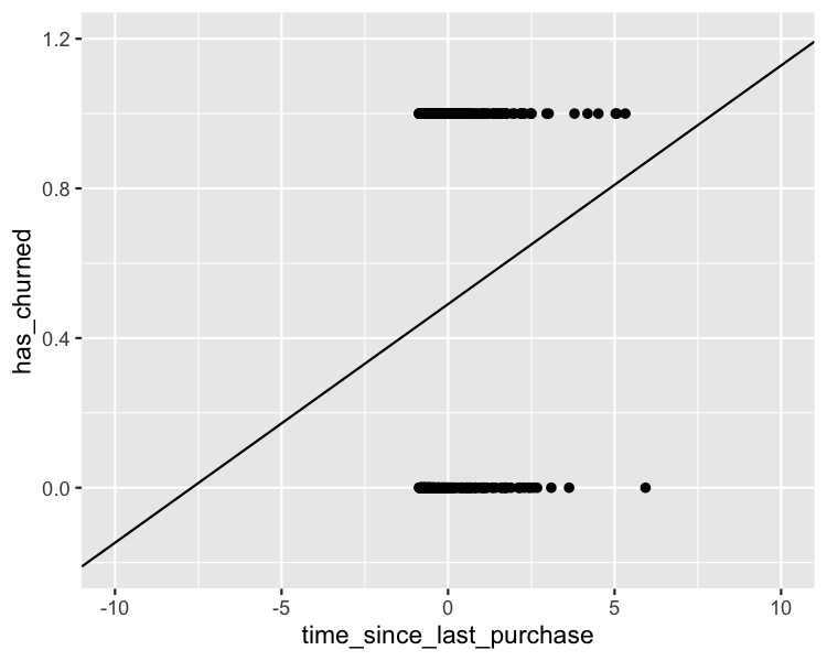
The scatter plot of whether or not the customer churned versus time since last purchase. The axes are zoomed out compared to last time, showing that the trend line extends below y equals 0 and above y equals 1, which ought to be impossible.

What is logistic regression?

Another type of generalized linear model.
Used when the response variable is logical.
The responses follow logistic (S-shaped) curve.

Linear regression using glm()

glm(has_churned ~ time_since_last_purchase, data = churn, family = gaussian)

Call:  glm(formula = has_churned ~ time_since_last_purchase, family = gaussian, 
    data = churn)

Coefficients:
             (Intercept)  time_since_last_purchase  
                 0.49078                   0.06378  

Degrees of Freedom: 399 Total (i.e. Null);  398 Residual
Null Deviance:        100 
Residual Deviance: 98.02     AIC: 578.7

Logistic regression: glm() with binomial family

mdl_recency_glm <- glm(has_churned ~ time_since_last_purchase, data = churn, family = binomial)

Call:  glm(formula = has_churned ~ time_since_last_purchase, family = binomial, 
    data = churn)

Coefficients:
             (Intercept)  time_since_last_purchase  
                -0.03502                   0.26921  

Degrees of Freedom: 399 Total (i.e. Null);  398 Residual
Null Deviance:        554.5 
Residual Deviance: 546.4     AIC: 550.4

Visualizing the logistic model

ggplot(
  churn, 
  aes(time_since_last_purchase, has_churned)
) +
  geom_point() +
  geom_abline(
    intercept = intercept, slope = slope
  ) +
  geom_smooth(
    method = "glm", 
    se = FALSE, 
    method.args = list(family = binomial)
  )

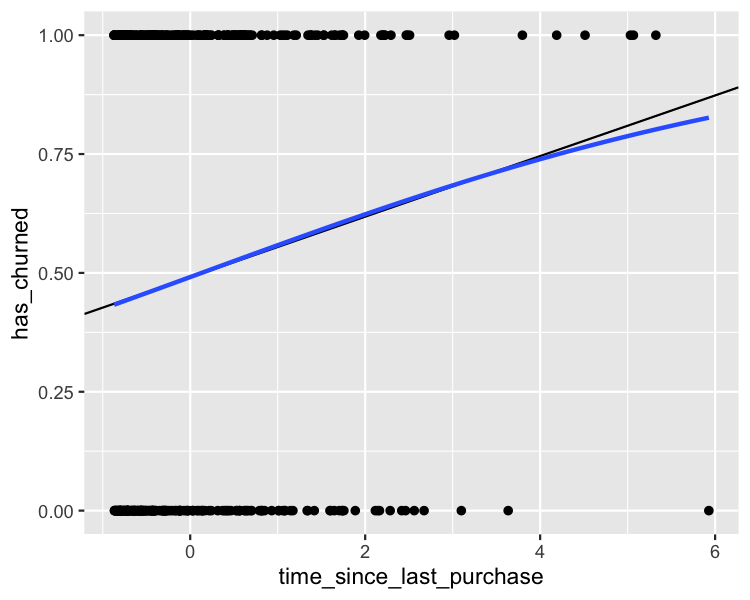
A scatter plot of whether or not the customer churned versus time since last purchase. Linear and logistic trend lines are shown, and both show increasing churn probabilities as time since last purchase increases. The two trend lines track each other quite closely except at high time since last purchase.

Zooming out

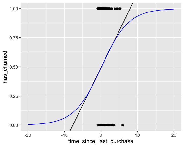
The scatter plot of whether or not the customer churned versus time since last purchase, with both trend lines. The axes are zoomed out compared to last time, showing that the logistic trend line never goes outside the zero to one churn range.

Let's practice!

Nhập môn Hồi quy bằng R