Transformace pro stabilizaci rozptylu
Forecasting v R

Rob J. Hyndman
Professor of Statistics at Monash University
Stabilizace rozptylu
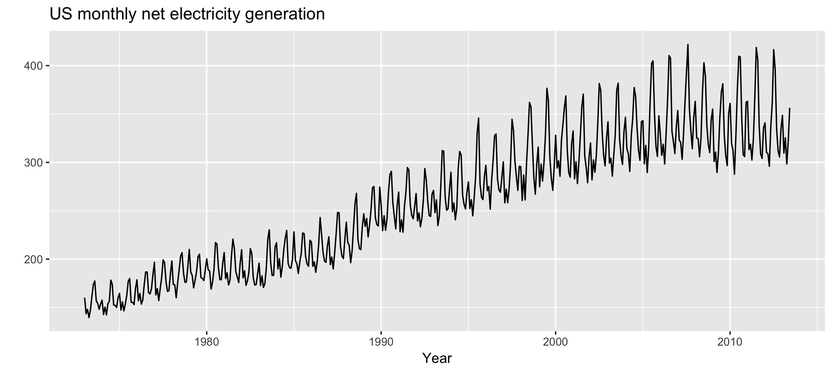
autoplot(usmelec) +
  xlab("Year") + ylab("") +
  ggtitle("US monthly net electricity generation")
Stabilizace rozptylu
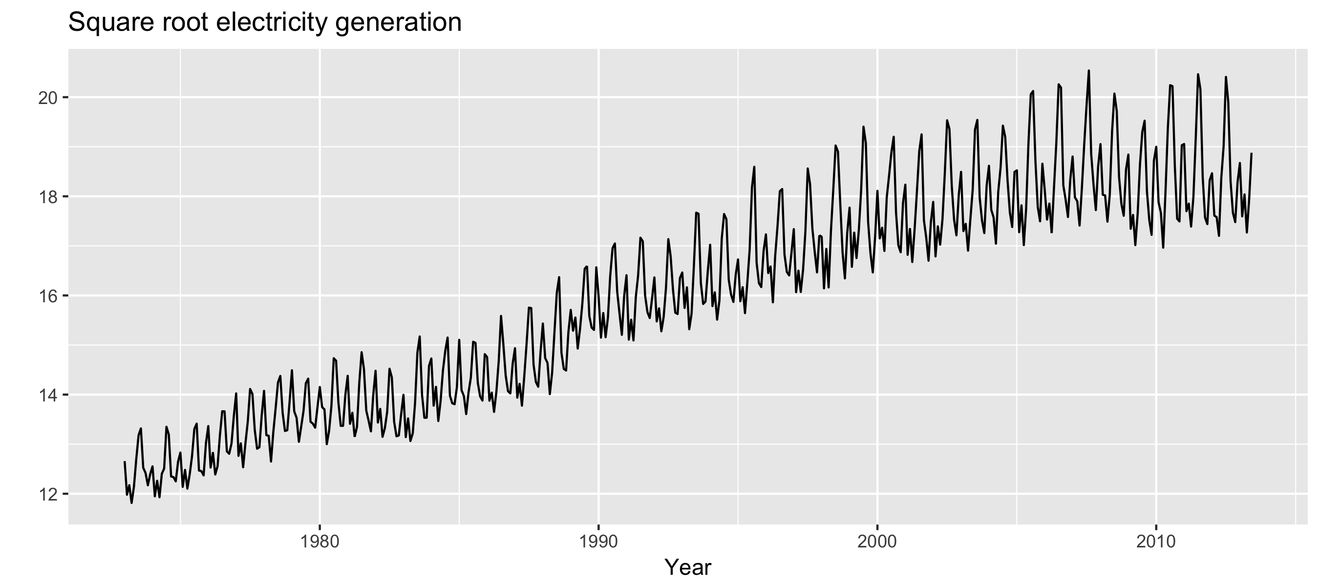
autoplot(usmelec^0.5) +
  xlab("Year") + ylab("") +
  ggtitle("Square root electricity generation")
Stabilizace rozptylu
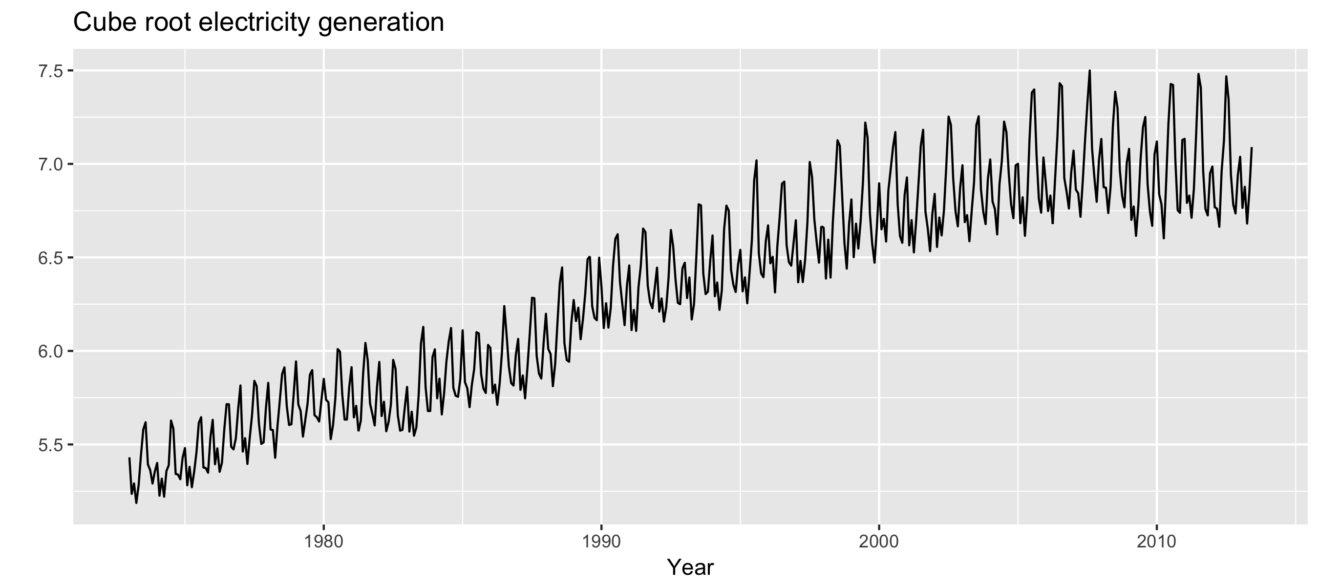
autoplot(usmelec^0.33333) +
  xlab("Year") + ylab("") +
  ggtitle("Cube root electricity generation")
Stabilizace rozptylu
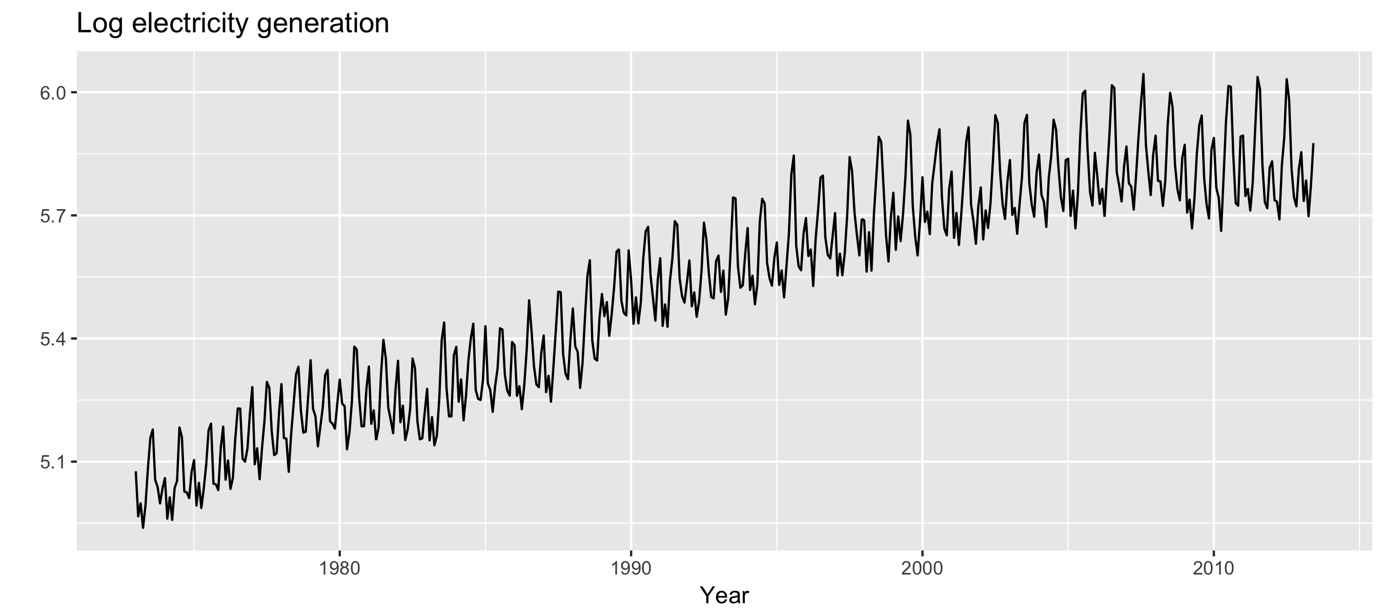
autoplot(log(usmelec)) +
  xlab("Year") + ylab("") +
  ggtitle("Log electricity generation")
Stabilizace rozptylu
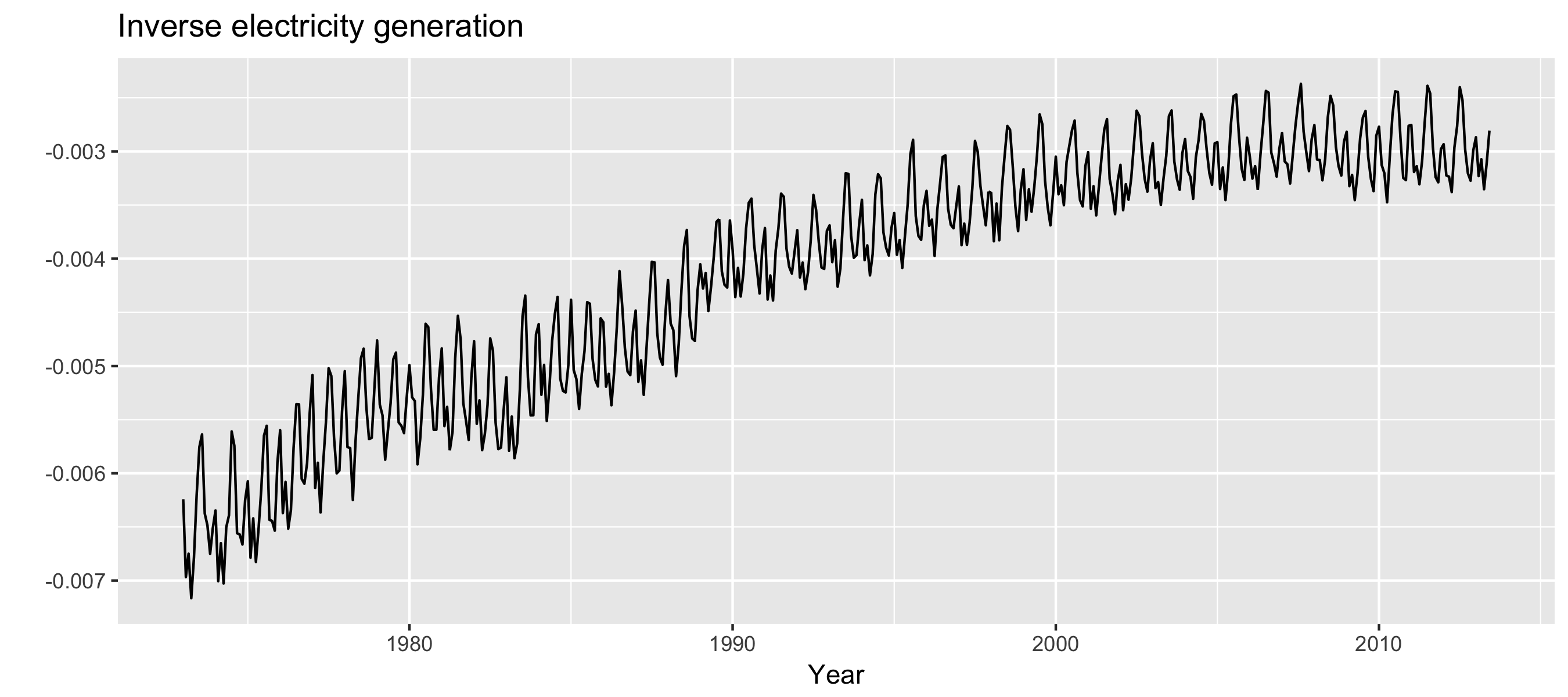
autoplot(-1/usmelec) +
  xlab("Year") + ylab("") +
  ggtitle("Inverse electricity generation")
Zpětná transformace
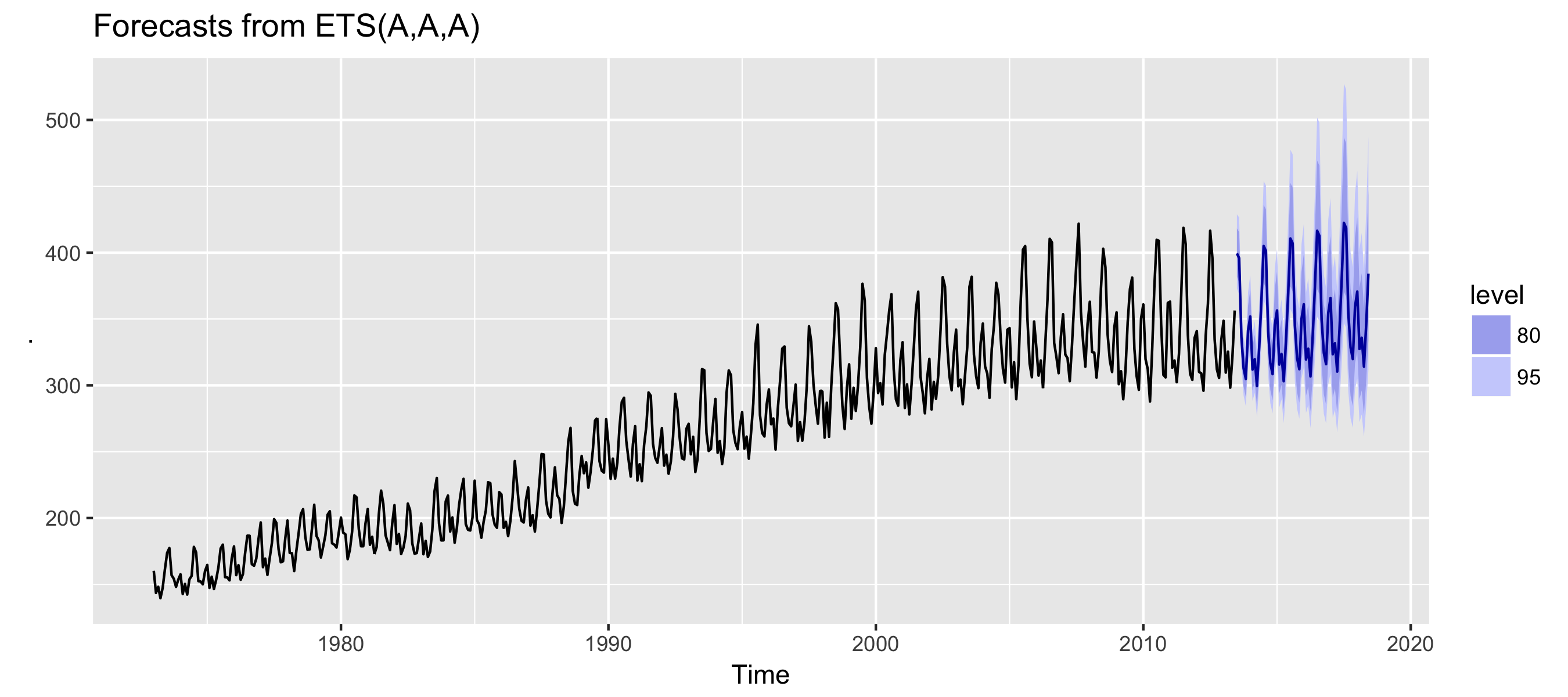
usmelec %>%
  ets(lambda = -0.57) %>%
  forecast(h = 60) %>%
  autoplot()