Dynamická regrese

Forecasting v R

Rob J. Hyndman

Professor of Statistics at Monash University

Dynamická regrese

Regresní model s chybami ARIMA:

$y_t = \beta_0 + \beta_1 x_{1,t} + ... + \beta_r x_{r,t} + e_t$

  • $y_t$ modelováno jako funkce r vysvětlujících proměnných $\ x_{1,t},...,x_{r,t}$
Forecasting v R

Dynamická regrese

Regresní model s chybami ARIMA:

$y_t = \beta_0 + \beta_1 x_{1,t} + ... + \beta_r x_{r,t} + e_t \leftarrow$

  • $y_t$ modelováno jako funkce r vysvětlujících proměnných $\ x_{1,t},...,x_{r,t}$
  • V dynamické regresi může být $e_t$ procesem ARIMA
Forecasting v R

Dynamická regrese

Regresní model s chybami ARIMA:

$y_t = \beta_0 + \beta_1 x_{1,t} + ... + \beta_r x_{r,t} + e_t$

  • $y_t$ modelováno jako funkce r vysvětlujících proměnných $\ x_{1,t},...,x_{r,t}$
  • V dynamické regresi může být $e_t$ procesem ARIMA
  • V klasické regresi se předpokládá, že $e_t$ je bílý šum
Forecasting v R

Osobní spotřeba a příjmy v USA

autoplot(uschange[,1:2], facets = TRUE) +
  xlab("Year") + ylab("") +
  ggtitle("Quarterly changes in US consumption
          and personal income")
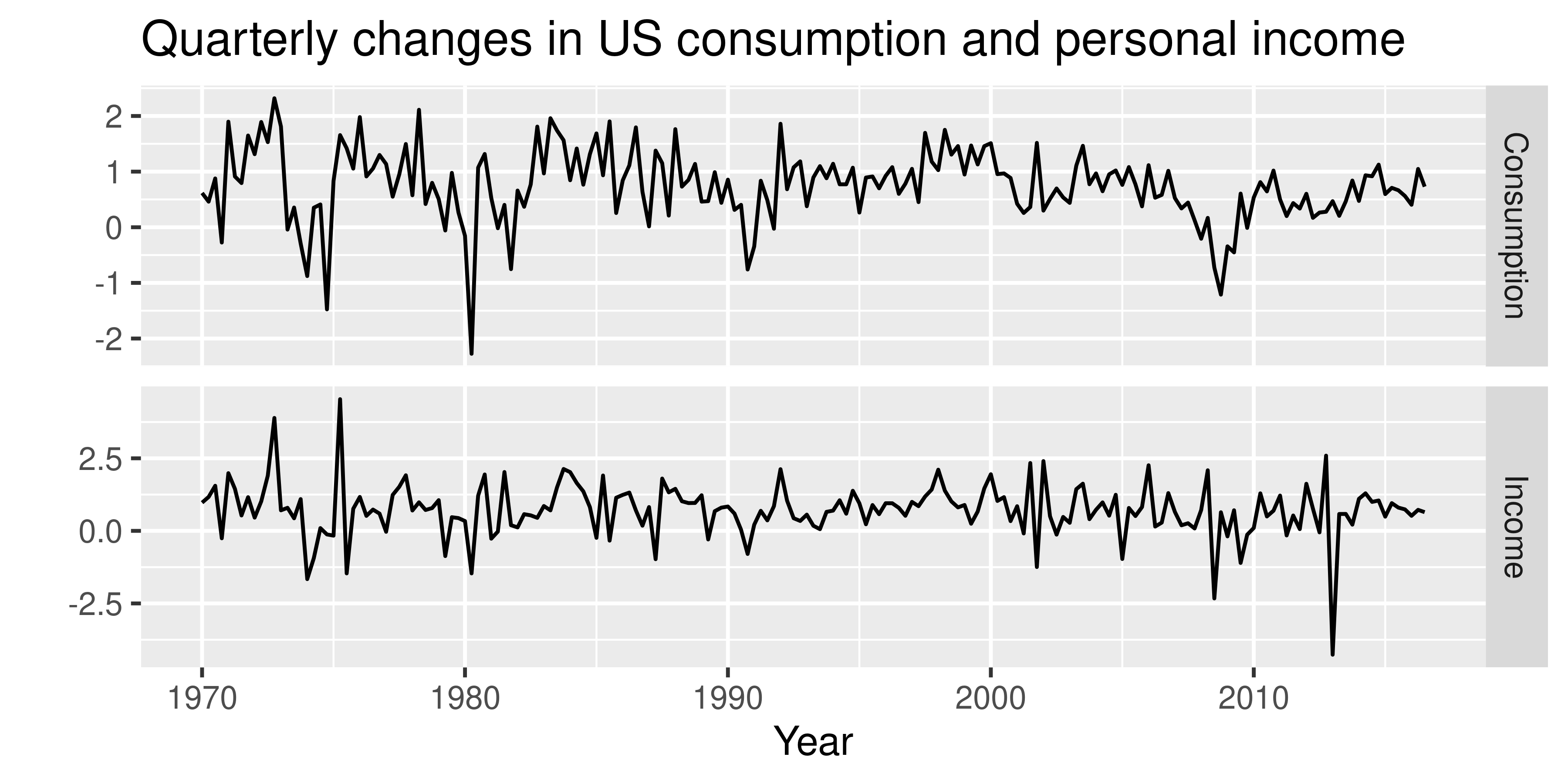
Čtvrtletní změny spotřeby a osobního příjmu v USA

Forecasting v R

Osobní spotřeba a příjmy v USA

ggplot(aes(x = Income, y = Consumption),
           data = as.data.frame(uschange)) +
  geom_point() +
  ggtitle("Quarterly changes in US consumption and
          personal income")
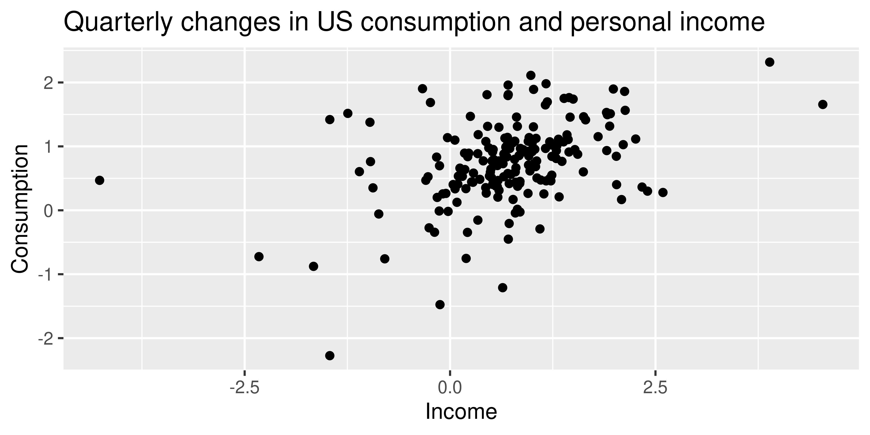
Bodový graf čtvrtletních změn spotřeby a příjmů v USA

Forecasting v R

Dynamický regresní model osobní spotřeby v USA

fit <- auto.arima(uschange[,"Consumption"],
                  xreg = uschange[,"Income"])
fit
Series: uschange[, "Consumption"]
Regression with ARIMA(1,0,2) errors
Coefficients:
         ar1      ma1     ma2  intercept      xreg
      0.6922  -0.5758  0.1984     0.5990    0.2028
 s.e. 0.1159   0.1301  0.0756     0.0884    0.0461

sigma^2 = 0.3219:  log likelihood = -156.95
AIC=325.91  AICc=326.37    BIC=345.29
Forecasting v R

Rezidua dynamického regresního modelu

checkresiduals(fit)
Ljung-Box test
data:  Residuals from Regression with ARIMA(1,0,2) errors
Q* = 5.8916, df = 5, p-value = 0.3169
Model df: 3.   Total lags used: 8
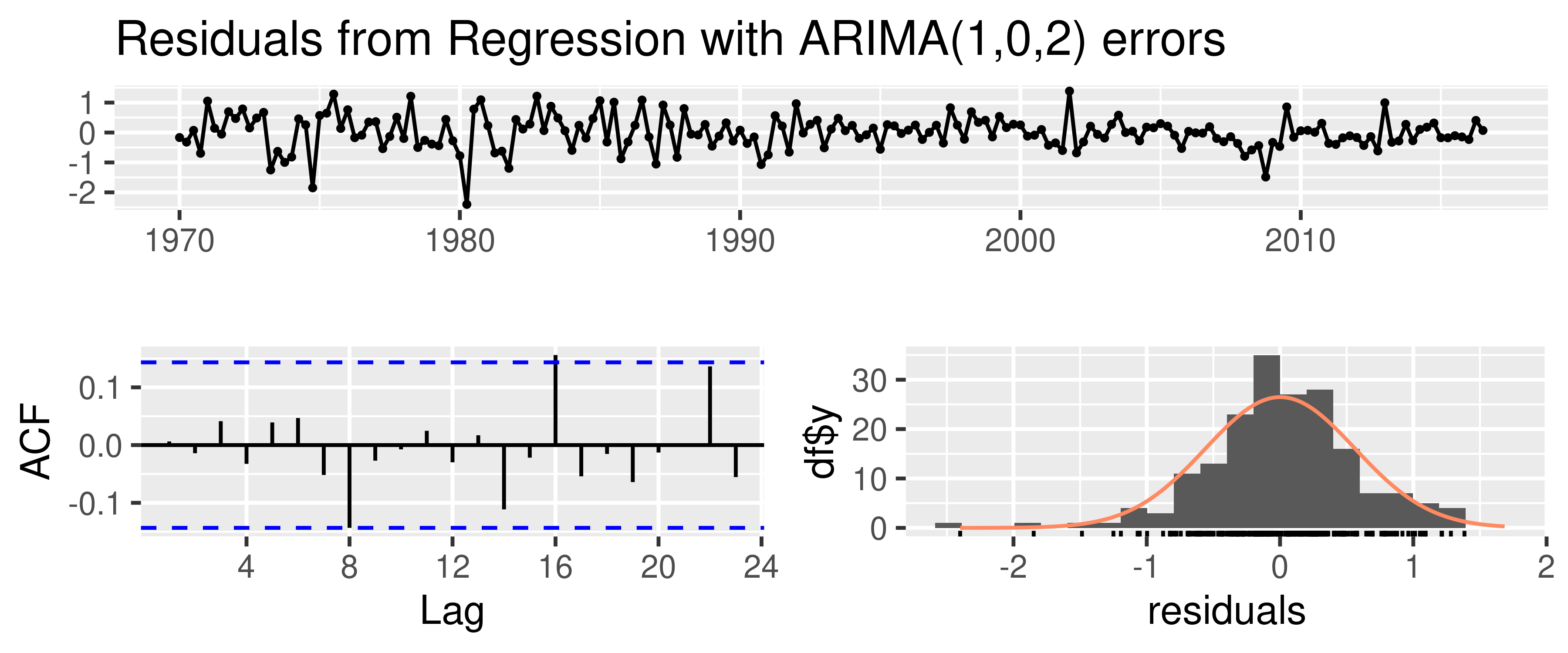
Rezidua dynamického regresního modelu

Forecasting v R

Prognózy dynamického regresního modelu

fcast <- forecast(fit, xreg = rep(0.8, 8))
autoplot(fcast) +
  xlab("Year") + ylab("Percentage change")
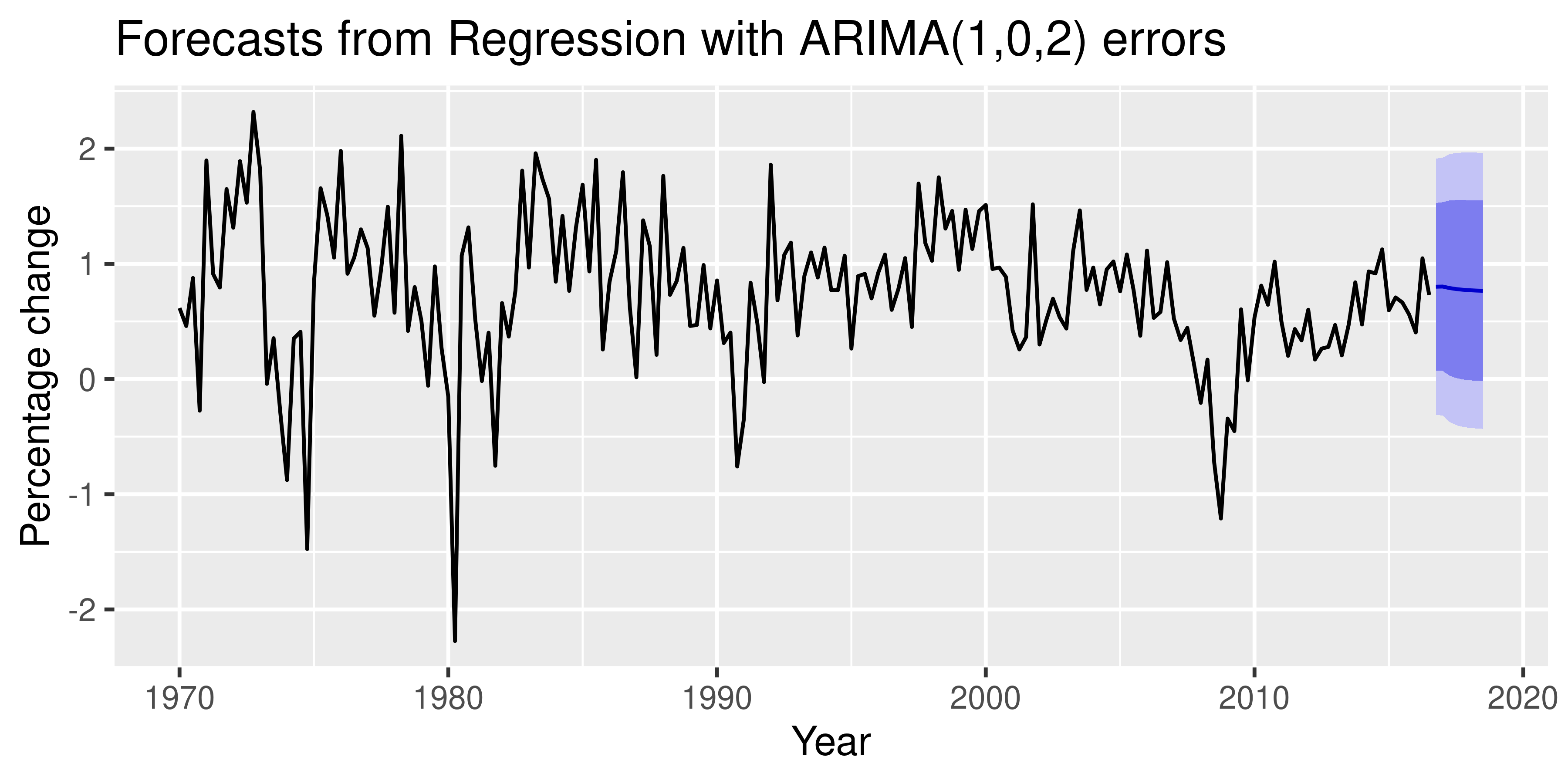
Prognózy dynamického regresního modelu

Forecasting v R

Pojďme si procvičit!

Forecasting v R

Preparing Video For Download...