Dynamická harmonická regrese
Forecasting v R

Rob J. Hyndman
Professor of Statistics at Monash University
Dynamická harmonická regrese

Dynamická harmonická regrese
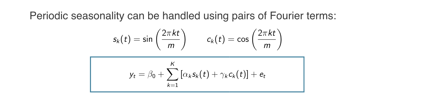
$m =$ sezónní perioda
Každou periodickou funkci lze pro dostatečně velké K aproximovat součty členů sin a cos
Regresní koeficienty: $\alpha_k$ a $\gamma_k$
$e_t$ lze modelovat jako nesezónní proces ARIMA
Předpokládá neměnný sezónní vzorec
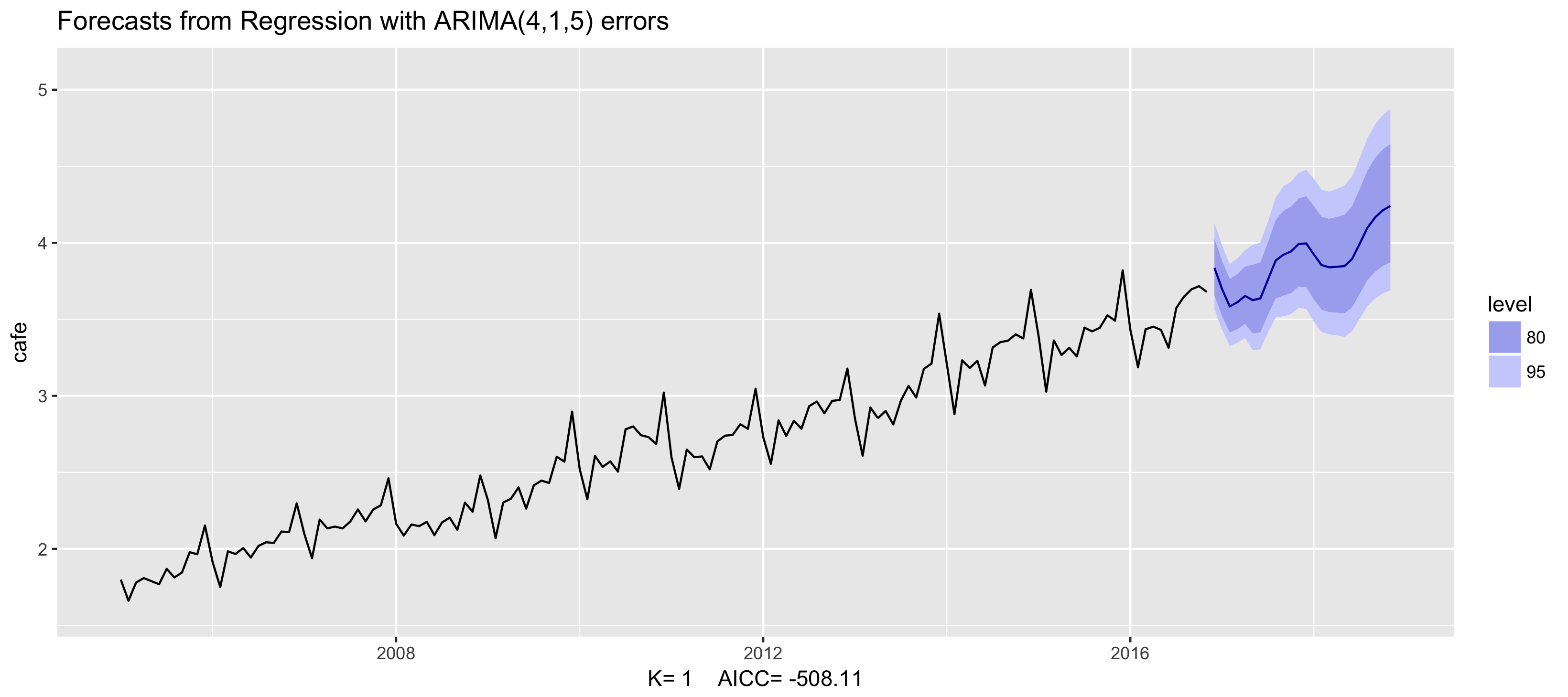
Příklad: výdaje v australských kavárnách
fit <- auto.arima(cafe, xreg = fourier(cafe, K = 1),
                  seasonal = FALSE, lambda = 0)
fit %>% forecast(xreg = fourier(cafe, K = 1, h = 24)) %>%
   autoplot() + ylim(1.6, 5.1)
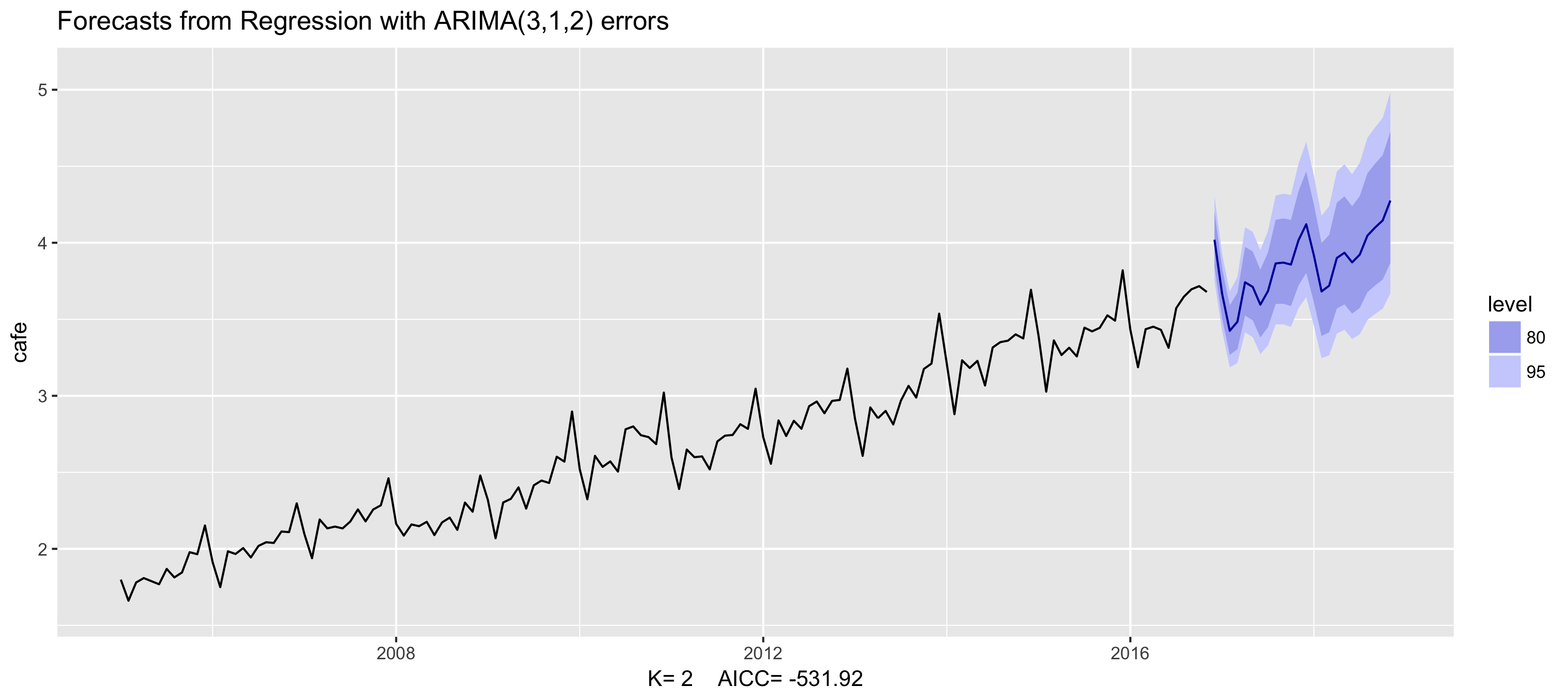
Příklad: výdaje v australských kavárnách
fit <- auto.arima(cafe, xreg = fourier(cafe, K = 2),
                  seasonal = FALSE, lambda = 0)
fit %>% forecast(xreg = fourier(cafe, K = 2, h = 24)) %>%
   autoplot() + ylim(1.6, 5.1)
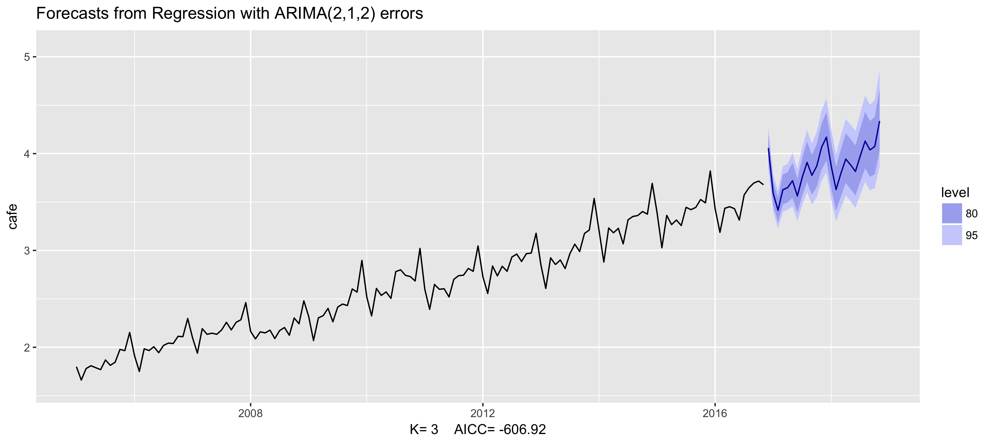
Příklad: výdaje v australských kavárnách
fit <- auto.arima(cafe, xreg = fourier(cafe, K = 3),
                  seasonal = FALSE, lambda = 0)
fit %>% forecast(xreg = fourier(cafe, K = 3, h = 24)) %>%
   autoplot() + ylim(1.6, 5.1)
Příklad: výdaje v australských kavárnách
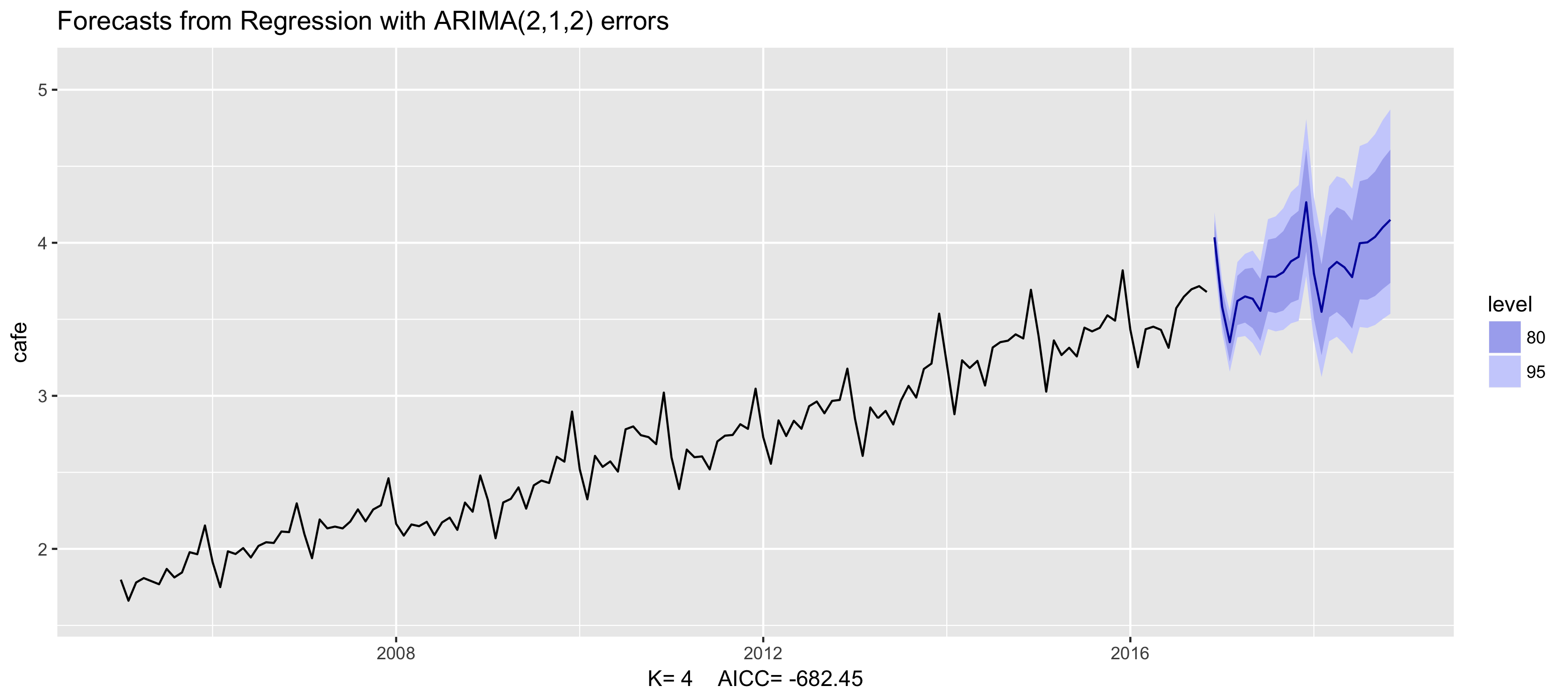
fit <- auto.arima(cafe, xreg = fourier(cafe, K = 4),
                  seasonal = FALSE, lambda = 0)
fit %>% forecast(xreg = fourier(cafe, K = 4, h = 24)) %>%
   autoplot() + ylim(1.6, 5.1)
Příklad: výdaje v australských kavárnách
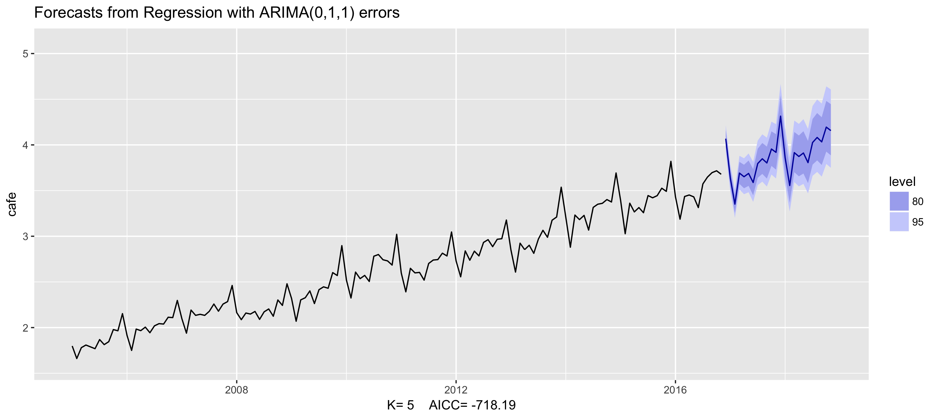
fit <- auto.arima(cafe, xreg = fourier(cafe, K = 5),
                  seasonal = FALSE, lambda = 0)
fit %>% forecast(xreg = fourier(cafe, K = 5, h = 24)) %>%
   autoplot() + ylim(1.6, 5.1)
Příklad: výdaje v australských kavárnách
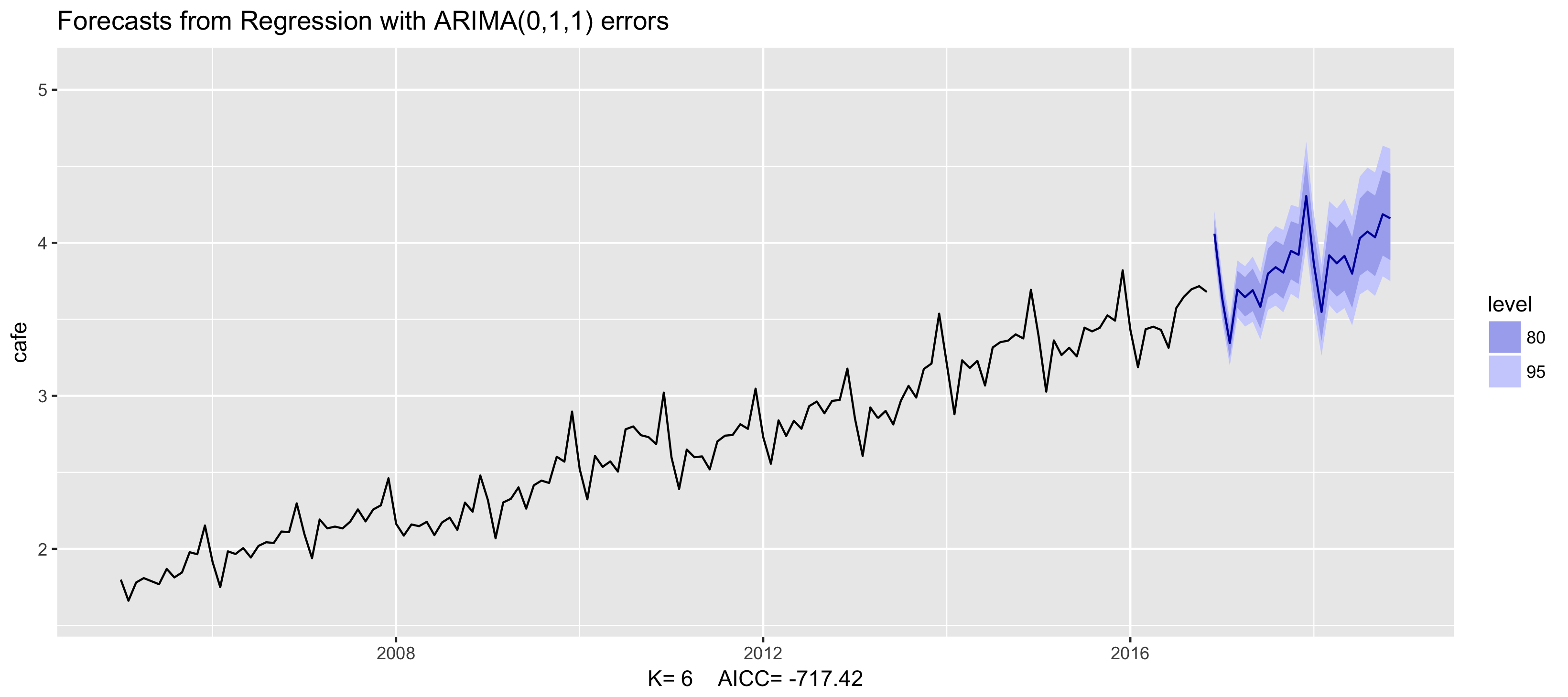
fit <- auto.arima(cafe, xreg = fourier(cafe, K = 6),
                  seasonal = FALSE, lambda = 0)
fit %>% forecast(xreg = fourier(cafe, K = 6, h = 24)) %>%
   autoplot() + ylim(1.6, 5.1)
Dynamická harmonická regrese

- Lze přidat další prediktory: $x_{t,1},...,x_{t,r}$
- K se volí minimalizací $AIC_c$
- K nesmí překročit m/2
- Zvláště vhodné pro týdenní, denní a subdennní data.

