Spojnicové grafy

Úvod do vizualizace dat s ggplot2

Rick Scavetta

Founder, Scavetta Academy

Běžné typy grafů

Typ grafu	Možné geomy
Bodové grafy	points, jitter, abline, smooth, count
Sloupcové grafy	histogram, bar, col, errorbar
Spojnicové grafy	line, path

Bobr

str(beaver)

'data.frame':    101 obs. of  3 variables:
 $ time  : POSIXct, format: "2000-01-01 09:30:00" "2000-01-01 09:40:00" "2000-01-01 09:50:00" ...
 $ temp  : num  36.6 36.7 36.9 37.1 37.2 ...
 $ active: Factor w/ 2 levels "0","1": 1 1 1 1 1 1 1 1 1 1 ...

Bobr

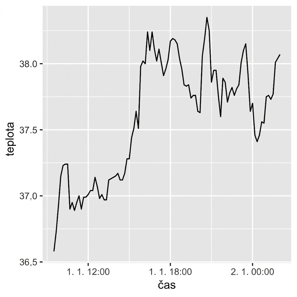
ggplot(beaver, aes(x = time, y = temp)) +
  geom_line()

Bobr

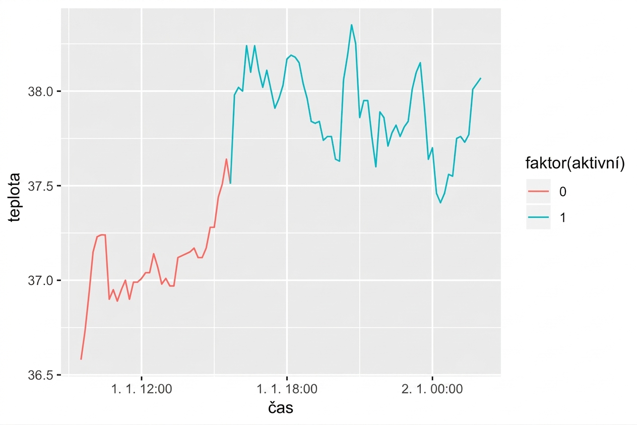
ggplot(beaver, aes(x = time, y = temp, 
                   color = factor(active))
                   ) +
  geom_line()

Datová sada úlovků ryb

str(fish)

'data.frame':    427 obs. of  3 variables:
 $ Species: Factor w/ 7 levels "Pink","Chum",..: 1 2 3 4 5 6 7 1 2 3 ...
 $ Year   : int  1950 1950 1950 1950 1950 1950 1950 1951 1951 1951 ...
 $ Capture: int  100600 139300 64100 30500 0 23200 10800 259000 155900 51200 ...

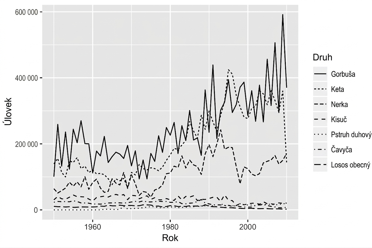
Estetika linetype

ggplot(fish, aes(x = Year, 
                 y = Capture, 
                 linetype = Species)) + 
  geom_line()

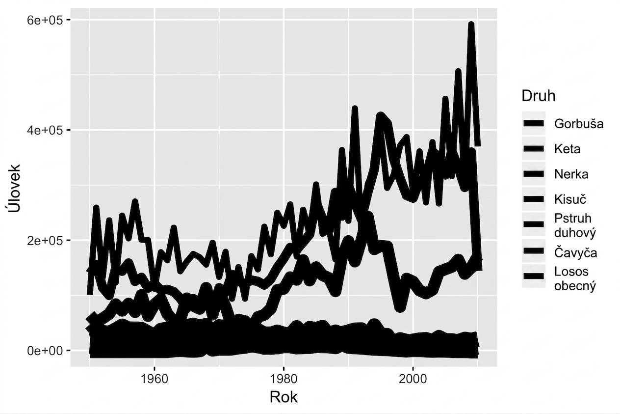
Estetika size

ggplot(fish, aes(x = Year, 
                 y = Capture, 
                 size = Species)) + 
  geom_line()

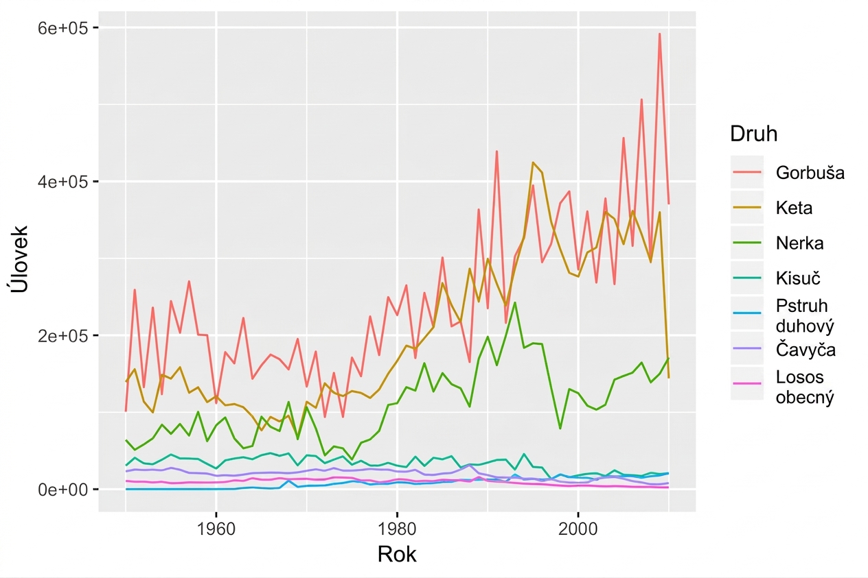
Estetika color

ggplot(fish, aes(x = Year, 
                 y = Capture, 
                 color = Species)) + 
  geom_line()

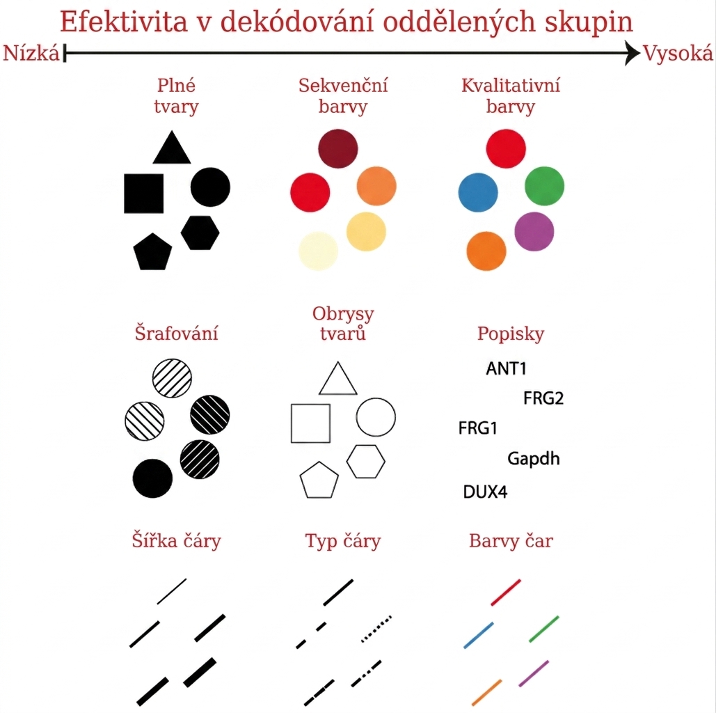
Estetika pro kategorické proměnné

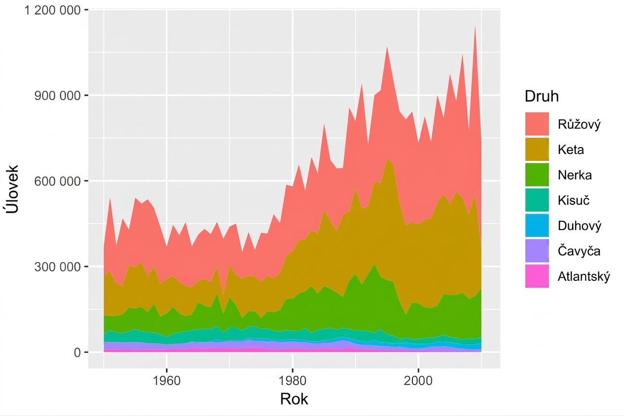
Estetika fill s geom_area()

ggplot(fish, aes(x = Year, 
                 y = Capture, 
                 fill = Species)) + 
  geom_area()

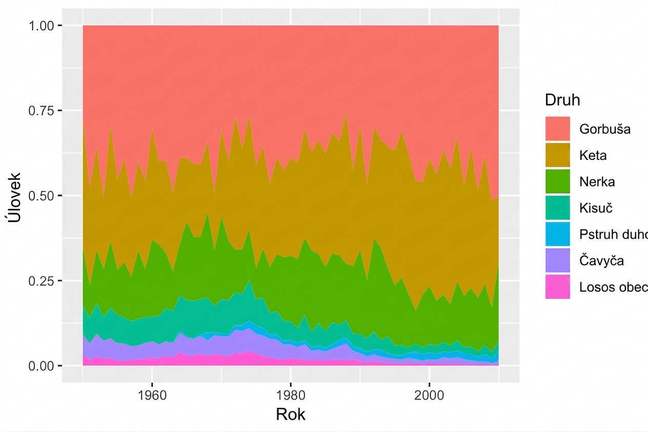
Použití position = "fill"

ggplot(fish, aes(x = Year, 
                 y = Capture, 
                 fill = Species)) + 
  geom_area(position = "fill")

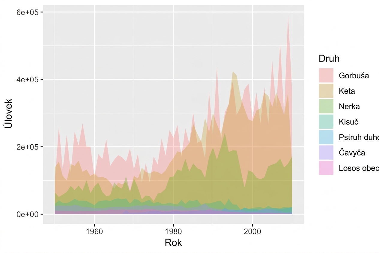
geom_ribbon()

ggplot(fish, aes(x = Year, 
                 y = Capture, 
                 fill = Species)) + 
  geom_ribbon(aes(ymax = Capture, 
                  ymin = 0), 
              alpha = 0.3)

Pojďme procvičovat!

Úvod do vizualizace dat s ggplot2