Testy hipotez i wyniki z

Testowanie hipotez w R

Richie Cotton

Data Evangelist at DataCamp

Testowanie A/B

Electronic Arts (EA) to firma produkująca gry wideo.
W 2013 roku wydała SimCity 5.
Jej celem było zwiększenie liczby zamówień przedsprzedażowych.
Zastosowała testy A/B do testowania różnych scenariuszy reklamowych.
Polega to na podziale użytkowników na grupy kontrolną i eksperymentalną.

Budynek Electronic Arts

¹ Źródło zdjęcia: „Electronic Arts" by majaX1 CC BY-NC-SA 2.0

Retail webpage A/B test

Control

SimCity webpage with banner that says "pre-order and get $20 off your next purchase"

Treatment

SimCity webpage without banner

A/B test results

The treatment group (no ad) got 43.4% more purchases than the control group (with ad).
The intuition that "showing an ad would increase sales" was completely wrong.
Was this result statistically significant or just by chance?
You need EA's data to determine this.
You'd use techniques from Sampling in R + this course to do so.

Ankieta Stack Overflow dla deweloperów 2020

library(dplyr)
glimpse(stack_overflow)

Rows: 2,261
Columns: 8
$ respondent         <dbl> 36, 47, 69, 125, 147, 152, 166, 170, 187, 196, 221,…
$ age_first_code_cut <chr> "adult", "child", "child", "adult", "adult", "adult…
$ converted_comp     <dbl> 77556, 74970, 594539, 2000000, 37816, 121980, 48644…
$ job_sat            <fct> Slightly satisfied, Very satisfied, Very satisfied,…
$ purple_link        <chr> "Hello, old friend", "Hello, old friend", "Hello, o…
$ age_cat            <chr> "At least 30", "At least 30", "Under 30", "At least…
$ age                <dbl> 34, 53, 25, 41, 28, 30, 28, 26, 43, 23, 24, 35, 37,…
$ hobbyist           <chr> "Yes", "Yes", "Yes", "Yes", "No", "Yes", "Yes", "Ye…

Formułowanie hipotezy o średniej

Hipoteza:

Średnie roczne wynagrodzenie populacji data scientistów wynosi 110 000 USD.

Estymator punktowy (statystyka próby):

mean_comp_samp <- mean(stack_overflow$converted_comp)

mean_comp_samp <- stack_overflow %>% 
  summarize(mean_compensation = mean(converted_comp)) %>% 
  pull(mean_compensation)

119574.7

Generowanie rozkładu bootstrapowego

# Krok 3. Powtórz kroki 1 i 2 wiele razy
so_boot_distn <- replicate(
  n = 5000,
  expr = {

    # Krok 1. Ponowne próbkowanie
    stack_overflow %>%
      slice_sample(prop = 1, replace = TRUE) %>%

      # Krok 2. Oblicz estymator punktowy
      summarize(mean_compensation = mean(converted_comp)) %>% 
      pull(mean_compensation)

}
)

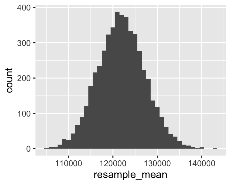
¹ Rozkłady bootstrapowe są omawiane w rozdziale 4 kursu Sampling in R

Wizualizacja rozkładu bootstrapowego

tibble(resample_mean = so_boot_distn) %>%
  ggplot(aes(resample_mean)) +
  geom_histogram(binwidth = 1000)

Histogram rozkładu bootstrapowego – ma kształt dzwonu i rozciąga się mniej więcej od 110 000 do 140 000

Błąd standardowy

std_error <- sd(so_boot_distn)

5511.674

Wyniki z

$\text{wartość standaryzowana} = \dfrac{\text{wartość} - \text{średnia}}{\text{odchylenie standardowe}}$

$z = \dfrac{\text{stat. próby} - \text{wart. param. hip.}}{\text{błąd standardowy}}$

$z = \dfrac{\$119\,574{,}7 - \$110\,000}{\$5511{,}67} = 1{,}737$

mean_comp_samp

119574.7

mean_comp_hyp <- 110000

std_error

5511.674

z_score <- (mean_comp_samp - mean_comp_hyp) / std_error

1.737171

Testowanie hipotezy

Czy 1,737171 to wartość wysoka czy niska?
To właśnie cel tego kursu!

Zastosowanie testowania hipotez:

Określenie, czy statystyki próby są bliskie, czy odległe od oczekiwanych (lub „hipotetycznych") wartości.

Standardowy rozkład normalny (z)

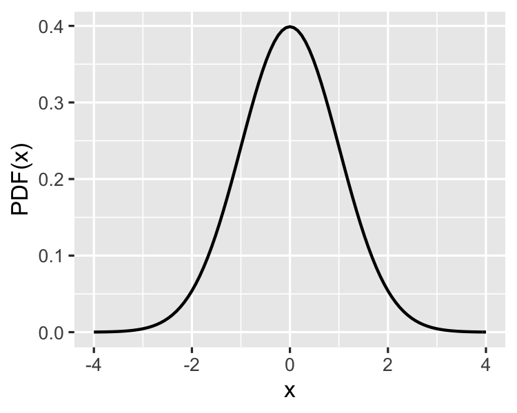
Standardowy rozkład normalny: rozkład normalny ze średnią zero i odchyleniem standardowym 1.

tibble(x = seq(-4, 4, 0.01)) %>% 
  ggplot(aes(x)) +
  stat_function(fun = dnorm) +
  ylab("PDF(x)")

Wykres gęstości PDF dla standardowego rozkładu normalnego

Let's practice!

Testowanie hipotez w R