Schemat walidacji na zbiorze walidacyjnym

Modelowanie danych w Tidyverse

Albert Y. Kim

Assistant Professor of Statistical and Data Sciences

Podejście ze zbiorem walidacyjnym

Użyj dwóch niezależnych zbiorów danych, aby:

Wytrenować/dopasować model
Ocenić zdolność predykcyjną modelu, tj. zwalidować go

Podział na zbiór treningowy i testowy

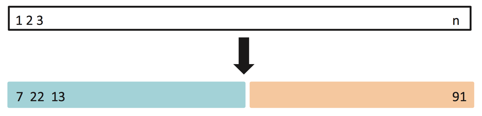
Losowo podziel wszystkie $n$ obserwacji (białe) na:

Zbiór treningowy (niebieski) do dopasowania modeli
Zbiór testowy (pomarańczowy) do generowania prognoz

Podział na zbiór treningowy i testowy w R

library(dplyr)

# Randomly shuffle order of rows:
house_prices_shuffled <- house_prices %>% 
  sample_frac(size = 1, replace = FALSE)


# Split into train and test:
train <- house_prices_shuffled %>%
  slice(1:10000)
test <- house_prices_shuffled %>%
  slice(10001:21613)

Trenowanie modeli na danych treningowych

train_model_price_1 <- lm(log10_price ~ log10_size + yr_built,
                          data = train)

get_regression_table(train_model_price_1)

# A tibble: 3 x 7
  term       estimate std_error statistic p_value lower_ci...
  <chr>         <dbl>     <dbl>     <dbl>   <dbl>    <dbl>...
1 intercept     5.34      0.111      48.3       0    5.13...
2 log10_size    0.923     0.009      97.5       0    0.905...
3 yr_built     -0.001     0         -23.0       0   -0.001...

Generowanie prognoz na danych testowych

# Train model on train:
train_model_price_1 <- lm(log10_price ~ log10_size + yr_built,
                          data = train)

# Get predictions on test:
get_regression_points(train_model_price_1, newdata = test)

# A tibble: 11,613 x 6
      ID log10_price log10_size yr_built log10_price_hat...
   <int>       <dbl>      <dbl>    <dbl>           <dbl>...
 1     1        5.83       3.29     1951            5.71...
 2     2        5.88       3.40     1922            5.84...
 3     3        6.15       3.67     2002            5.99...
 4     4        5.62       3        1953            5.43...
...
# ... with 11,603 more rows

Ocena prognoz za pomocą RMSE

# Train model:
train_model_price_1 <- lm(log10_price ~ log10_size + yr_built,
                          data = train)

# Get predictions and compute RMSE:
get_regression_points(train_model_price_1, newdata = test) %>%
  mutate(sq_residuals = residual^2) %>%
  summarize(rmse = sqrt(mean(sq_residuals)))

# A tibble: 1 x 1
   rmse
  <dbl>
1 0.165

Porównanie wartości RMSE

# Train model:
train_model_price_3 <- lm(log10_price ~ log10_size + condition,
                          data = train)

# Get predictions and compute RMSE:
get_regression_points(train_model_price_3, newdata = test) %>%
  mutate(sq_residuals = residual^2) %>%
  summarize(rmse = sqrt(mean(sq_residuals)))

# A tibble: 1 x 1
   rmse
  <dbl>
1 0.168

Ćwiczmy!

Modelowanie danych w Tidyverse