Ocena dopasowania modelu

Modelowanie z tidymodels w R

David Svancer

Data Scientist

Klasyfikacja binarna

Zmienna wynikowa z dwoma poziomami

Klasa pozytywna
- Zdarzenie, które chcemy przewidzieć
- "yes" w zmiennej purchased
Klasa negatywna
- "no"
W tidymodels zmienna wynikowa musi być czynnikiem (factor)
- Pierwszy poziom to klasa pozytywna
- Sprawdź kolejność za pomocą levels()

leads_df

# A tibble: 1,328 x 7
  purchased total_visits  ...   us_location
   <fct>        <dbl>     ...     <fct>
 1 yes            7       ...     west
 2 no             8       ...     west
 3 no             5       ...     southeast
# ... with 1,325 more rows

levels(leads_df[['purchased']])

[1] "yes" "no"

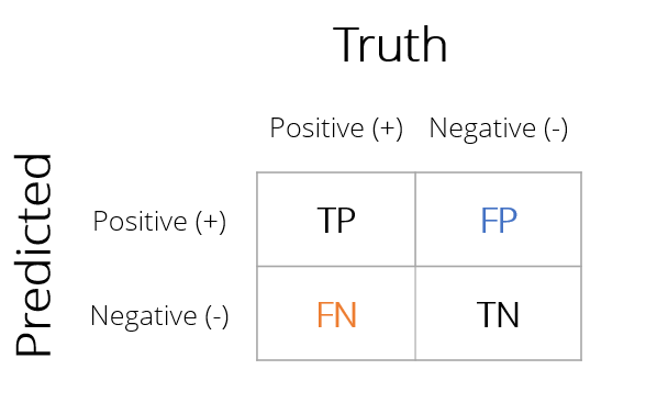
Macierz pomyłek

Macierz z liczbą wszystkich kombinacji rzeczywistych i przewidywanych wartości wynikowych

Poprawne przewidywania

Prawdziwy pozytyw (TP)
Prawdziwy negatyw (TN)

Błędy klasyfikacji

Fałszywy pozytyw (FP)
Fałszywy negatyw (FN)

Macierz pomyłek

Metryki klasyfikacji z yardstick

Tworzenie macierzy pomyłek i innych metryk dopasowania modelu z yardstick

Wymaga tabeli (tibble) z wynikami modelu zawierającej:
- Rzeczywiste wartości wynikowe
  - purchased
- Przewidywane kategorie wynikowe
  - .pred_class
- Szacowane prawdopodobieństwa każdej kategorii
  - .pred_yes
  - .pred_no

leads_results

# A tibble: 332 x 4
   purchased .pred_class .pred_yes .pred_no
   <fct>     <fct>           <dbl>    <dbl>
 1 no        no             0.134     0.866
 2 yes       yes            0.729     0.271
 3 no        no             0.133     0.867
 4 no        no             0.0916    0.908
 5 yes       yes            0.598     0.402
 6 no        no             0.128     0.872
 7 yes       no             0.112     0.888
 8 no        no             0.169     0.831
 9 no        no             0.158     0.842
10 yes       yes            0.520     0.480
# ... with 322 more rows

Macierz pomyłek z yardstick

Funkcja conf_mat()

Tabela (tibble) z wynikami modelu
truth - kolumna z rzeczywistymi wynikami
estimate - kolumna z przewidywanymi wynikami

Regresja logistyczna na leads_df

Poprawnie sklasyfikowano 252 z 332 klientów (76%)
46 fałszywych negatywów
34 fałszywe pozytywy

conf_mat(leads_results,

         truth = purchased,

         estimate = .pred_class)

          Truth
Prediction yes  no
       yes  74  34
       no   46 178

Dokładność klasyfikacji

Funkcja accuracy()

Przyjmuje te same argumenty co conf_mat()
Oblicza dokładność klasyfikacji

$$\frac{TP + TN}{TP + TN + FP + FN}$$

Funkcje yardstick zawsze zwracają tibble
- .metric - typ metryki
- .estimate - obliczona wartość

accuracy(leads_results, 
         truth = purchased, 
         estimate = .pred_class)

# A tibble: 1 x 3
  .metric  .estimator .estimate
  <chr>    <chr>          <dbl>
1 accuracy binary         0.759

Czułość (Sensitivity)

W wielu przypadkach dokładność nie jest najlepszą metryką

Dane leads_df
- Klasyfikowanie wszystkich jako 'no' daje 64% dokładności

Czułość (Sensitivity)

Odsetek wszystkich przypadków pozytywnych sklasyfikowanych poprawnie

Jaki odsetek klientów którzy dokonali zakupu model przewidział poprawnie?
- Mniej fałszywych negatywów zwiększa czułość

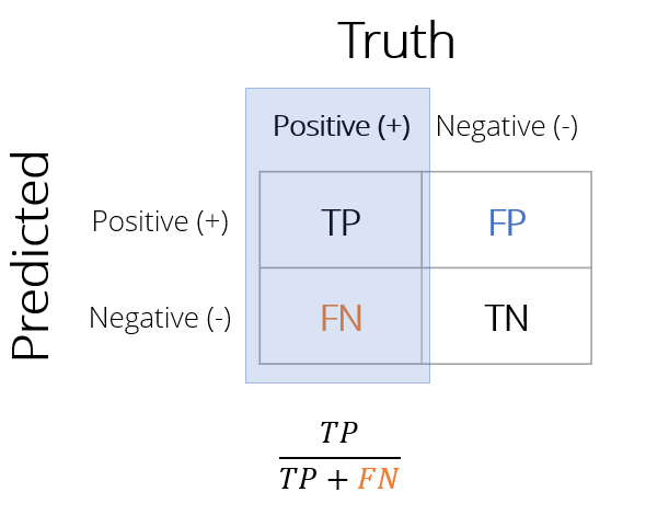
Obliczanie czułości

Funkcja sens()

Przyjmuje te same argumenty co conf_mat() i accuracy()
Zwraca wartość czułości w kolumnie .estimate

sens(leads_results, 
     truth = purchased, 
     estimate = .pred_class)

# A tibble: 1 x 3
  .metric .estimator .estimate
  <chr>   <chr>          <dbl>
1 sens    binary         0.617

Swoistość (Specificity)

Swoistość (Specificity) to odsetek wszystkich przypadków negatywnych sklasyfikowanych poprawnie

Jaki odsetek klientów którzy nie dokonali zakupu model przewidział poprawnie?
- Mniej fałszywych pozytywów zwiększa swoistość

1 - Swoistość

Inaczej: wskaźnik fałszywych pozytywów (FPR)
Odsetek fałszywych pozytywów wśród prawdziwych negatywów

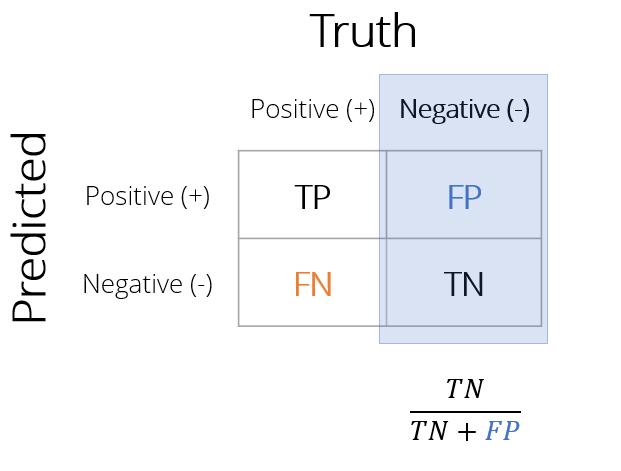
Obliczanie swoistości

Funkcja spec()

Przyjmuje te same argumenty co sens()
Zwraca wartość swoistości w kolumnie .estimate

spec(leads_results, 
     truth = purchased, 
     estimate = .pred_class)

# A tibble: 1 x 3
  .metric .estimator .estimate
  <chr>   <chr>          <dbl>
1 spec    binary         0.840

Tworzenie zestawu metryk

Własne zestawy metryk

Funkcja metric_set()
- Tworzy własną funkcję metryk z wybranych metryk yardstick
- Przekaż nazwy funkcji metryk yardstick do metric_set()
- Użyj własnej funkcji do obliczenia metryk

custom_metrics <-
  metric_set(accuracy, sens, spec)

custom_metrics(leads_results, 
               truth = purchased, 
               estimate = .pred_class)

# A tibble: 3 x 3
  .metric  .estimator .estimate
  <chr>    <chr>          <dbl>
1 accuracy binary         0.759
2 sens     binary         0.617
3 spec     binary         0.840

Wiele metryk

Metryki klasyfikacji binarnej

Szeroka gama metryk klasyfikacji binarnej
- accuracy(), kap(), sens(), spec(), ppv(), npv(), mcc(), j_index(), bal_accuracy(), detection_prevalence(), precision(), recall(), f_meas()
Przekaż wyniki conf_mat() do summary(), aby obliczyć wszystkie

https://yardstick.tidymodels.org/reference

conf_mat(leads_results, truth = purchased, 
         estimate = .pred_class) %>% 
  summary()

# A tibble: 13 x 3
   .metric              .estimator .estimate
   <chr>                <chr>          <dbl>
 1 accuracy             binary         0.759
 2 kap                  binary         0.466
 3 sens                 binary         0.617
 4 spec                 binary         0.840
 5 ppv                  binary         0.685
 6 npv                  binary         0.795
 7 mcc                  binary         0.468
 8 j_index              binary         0.456
 9 bal_accuracy         binary         0.728
10 detection_prevalence binary         0.325
11 precision            binary         0.685
12 recall               binary         0.617
13 f_meas               binary         0.649

Czas na ćwiczenia!

Modelowanie z tidymodels w R