Selekcja zmiennych na podstawie AUC

Modelowanie ryzyka kredytowego w R

Lore Dirick

Manager of Data Science Curriculum at Flatiron School

Krzywe ROC dla 4 modeli regresji logistycznej

Przycinanie na podstawie AUC

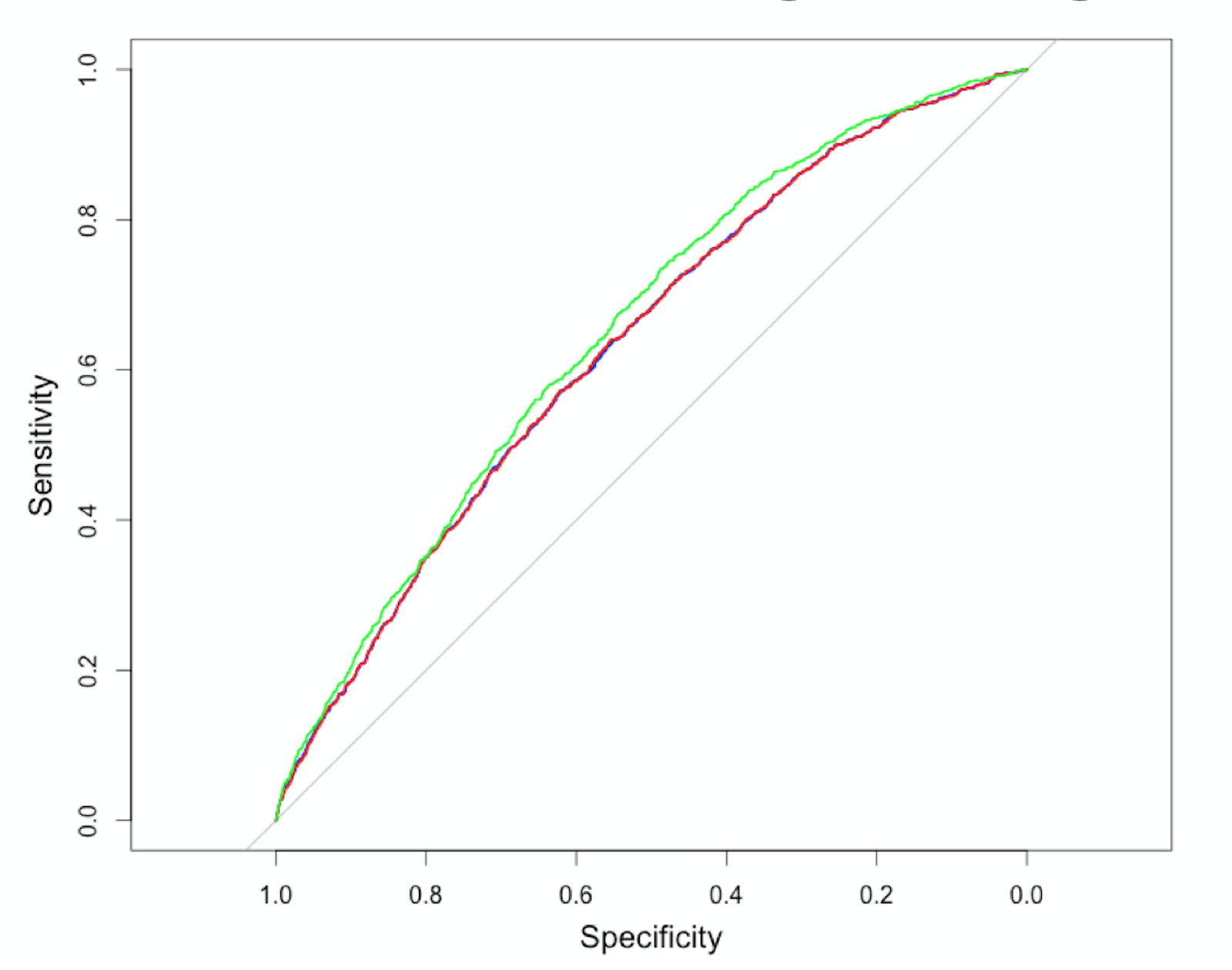
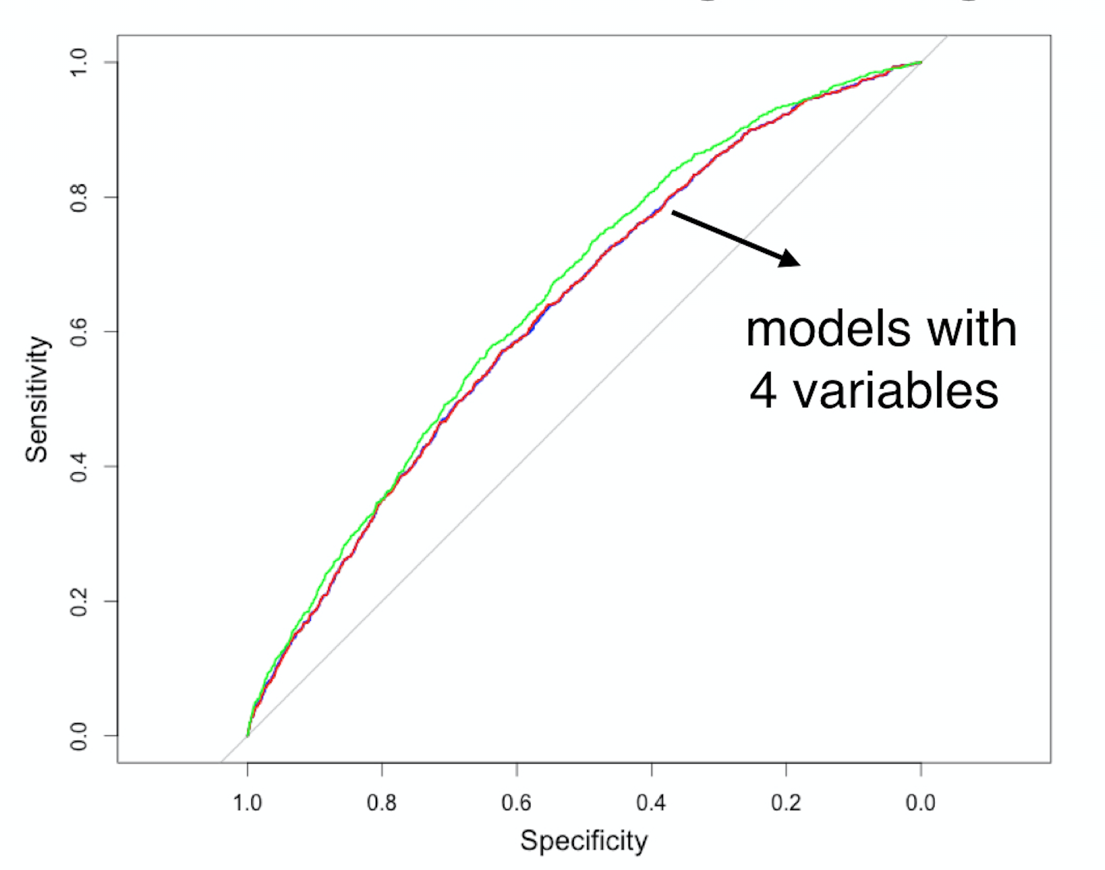
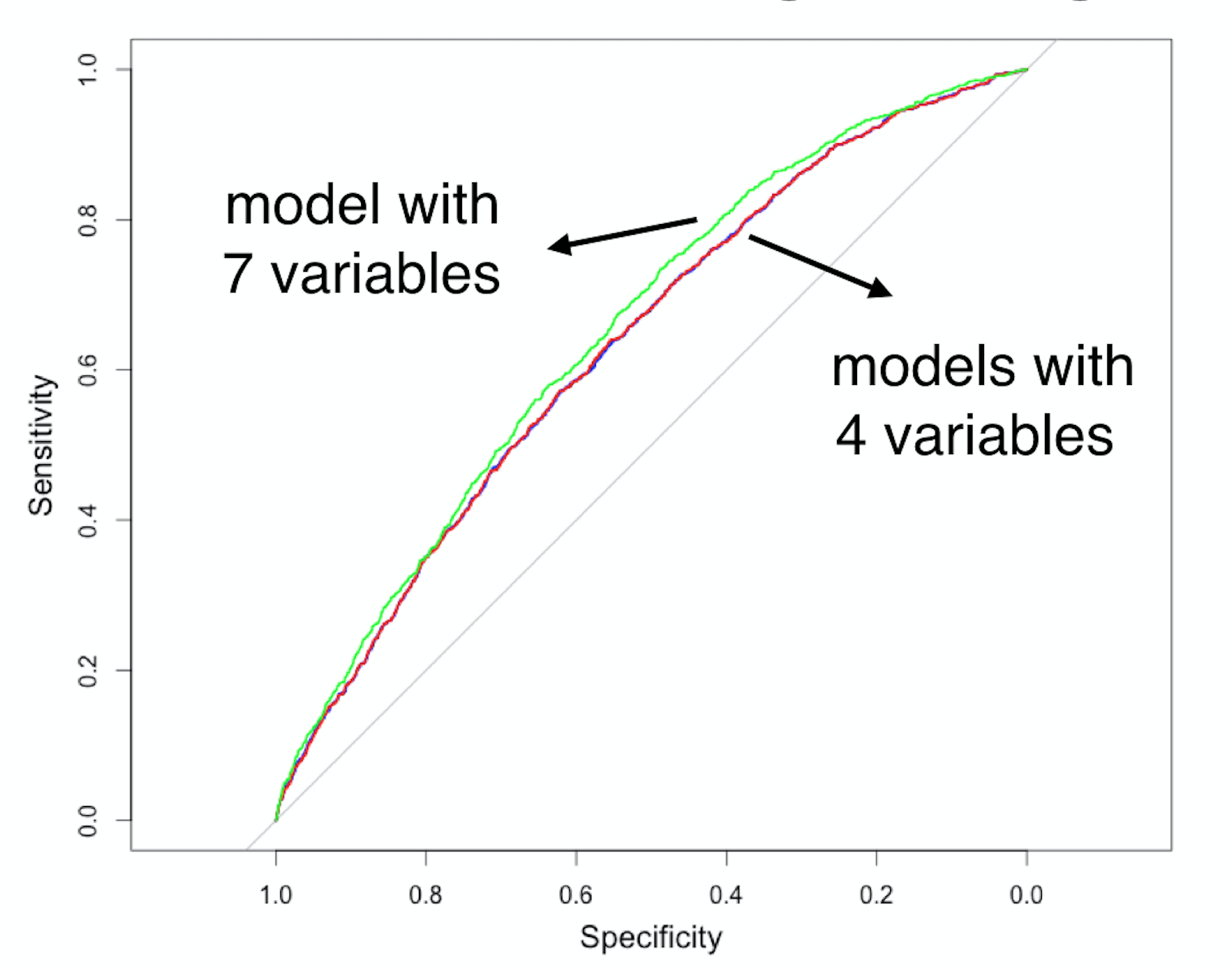
1) Zacząć od modelu zawierającego wszystkie zmienne (w tym przypadku 7) i obliczyć AUC

log_model_full <- glm(loan_status ~ loan_amnt + grade + home_ownership + 
                      annual_inc + age + emp_cat + ir_cat, 
                      family = "binomial", data = training_set)

predictions_model_full <- predict(log_model_full, 
                                  newdata = test_set, type ="response")

AUC_model_full <- auc(test_set$loan_status, predictions_model_full)

Area under the curve: 0.6512

2) Zbudować 7 nowych modeli, za każdym razem usuwając jedną zmienną, i obliczyć prognozy PD na zbiorze testowym

log_1_remove_amnt <- glm(loan_status ~ grade + home_ownership + annual_inc + age + emp_cat + ir_cat,
                         family = "binomial",
                         data = training_set)

log_1_remove_grade <- glm(loan_status ~ loan_amnt + home_ownership + annual_inc + age + emp_cat + ir_cat,
                          family = "binomial",
                          data = training_set)

log_1_remove_home <- glm(loan_status ~ loan_amnt + grade + annual_inc + age + emp_cat + ir_cat,
                         family = "binomial",
                         data = training_set)

pred_1_remove_amnt <- predict(log_1_remove_amnt, newdata = test_set, type = "response")
pred_1_remove_grade <- predict(log_1_remove_grade, newdata = test_set, type = "response")
pred_1_remove_home <- predict(log_1_remove_home, newdata = test_set, type = "response")
...

3) Zachować model z najlepszym AUC (AUC pełnego modelu: 0.6512)

auc(test_set$loan_status, pred_1_remove_amnt)

Area under the curve: 0.6537

auc(test_set$loan_status, pred_1_remove_grade)

Area under the curve: 0.6438

auc(test_set$loan_status, pred_1_remove_home)

Area under the curve: 0.6537

4) Powtarzać, aż AUC zacznie (znacząco) maleć

Czas na ćwiczenia!

Modelowanie ryzyka kredytowego w R