可视化数据

使用 pandas 进行数据处理

Maggie Matsui

Senior Content Developer at DataCamp

直方图

import matplotlib.pyplot as plt

dog_pack["height_cm"].hist()

plt.show()

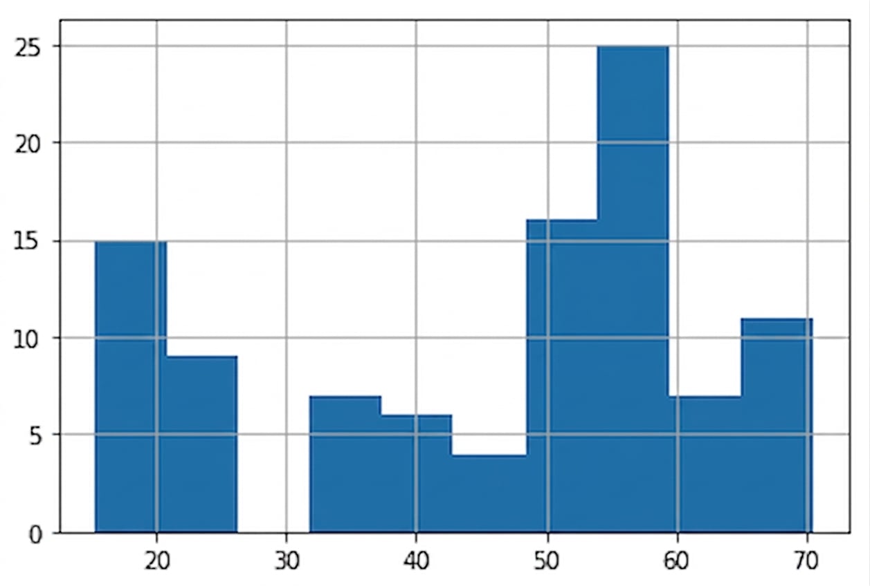
狗身高的直方图。最矮小的不足 20 cm，最高的为 70 cm。最常见的身高在 50–60 cm。

直方图

dog_pack["height_cm"].hist(bins=20)
plt.show()

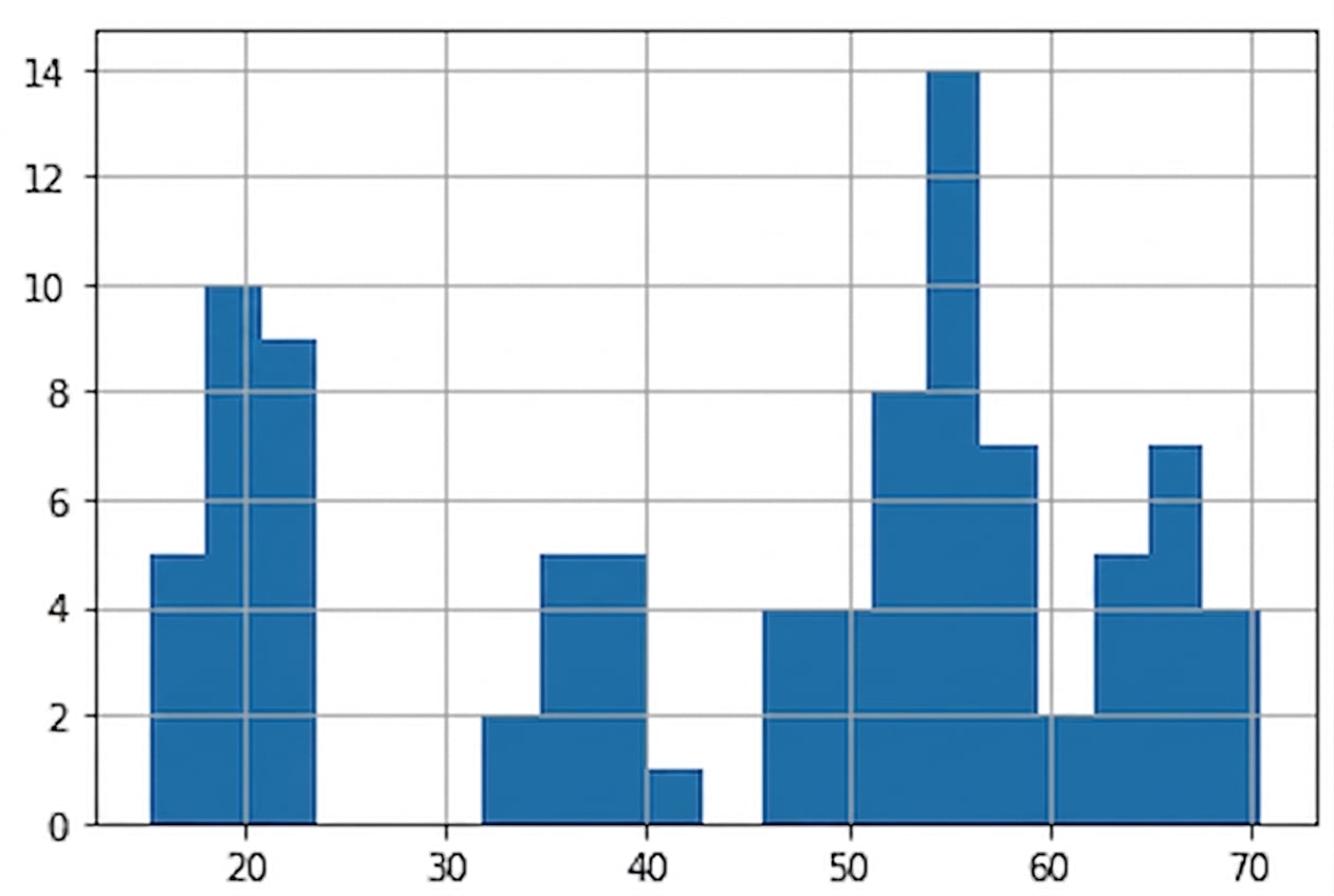
与前页相同的狗身高直方图，但有 20 个更窄的箱。

dog_pack["height_cm"].hist(bins=5)
plt.show()

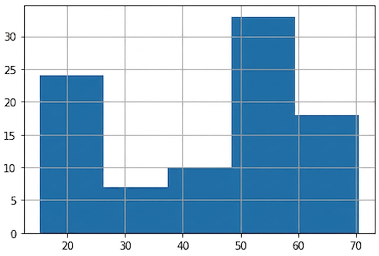
与前页相同的狗身高直方图，但只有 5 个更宽的箱。

条形图

avg_weight_by_breed = dog_pack.groupby("breed")["weight_kg"].mean()
print(avg_weight_by_breed)

breed
Beagle         10.636364
Boxer          30.620000
Chihuahua       1.491667
Chow Chow      22.535714
Dachshund       9.975000
Labrador       31.850000
Poodle         20.400000
St. Bernard    71.576923
Name: weight_kg, dtype: float64

条形图

avg_weight_by_breed.plot(kind="bar")

plt.show()

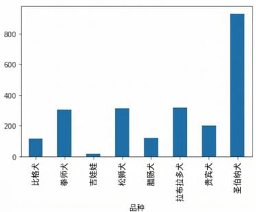
按品种划分的狗的平均体重（千克）的条形图。圣伯纳犬最重，吉娃娃最轻。

avg_weight_by_breed.plot(kind="bar",
    title="Mean Weight by Dog Breed")
plt.show()

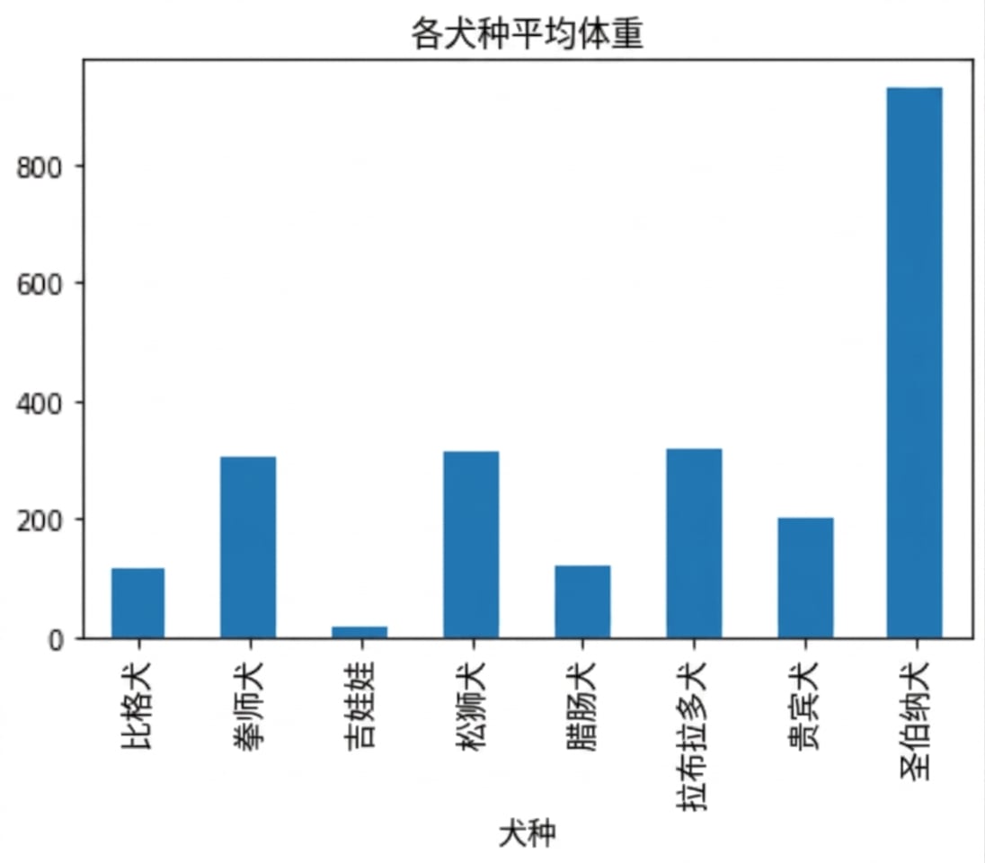
与左侧相同的条形图，但增加了标题"Mean Weight by Dog Breed"。

折线图

sully.head()

          date    weight_kg
0   2019-01-31         36.1
1   2019-02-28         35.3
2   2019-03-31         32.0
3   2019-04-30         32.9
4   2019-05-31         32.0

sully.plot(x="date", 
           y="weight_kg", 
           kind="line")
plt.show()

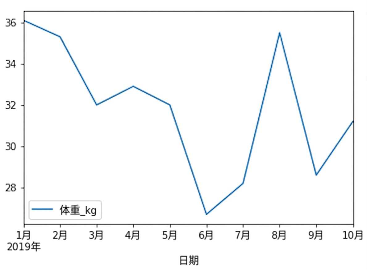
一条折线图，显示名为 Sully 的狗的体重随时间变化。体重在 27 到 36 千克之间波动。

旋转轴标签

sully.plot(x="date", y="weight_kg", kind="line", rot=45)
plt.show()

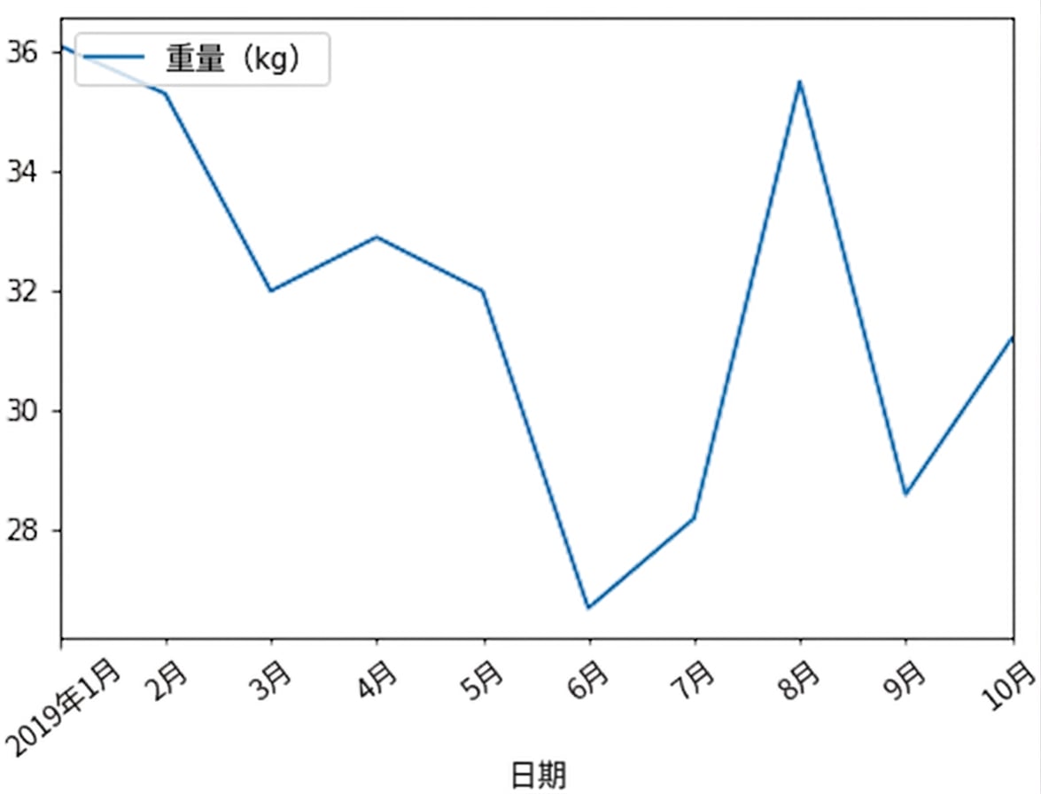
与上一页相同的 Sully 体重折线图，但 x 轴标签顺时针旋转 45 度。

散点图

dog_pack.plot(x="height_cm", y="weight_kg", kind="scatter")
plt.show()

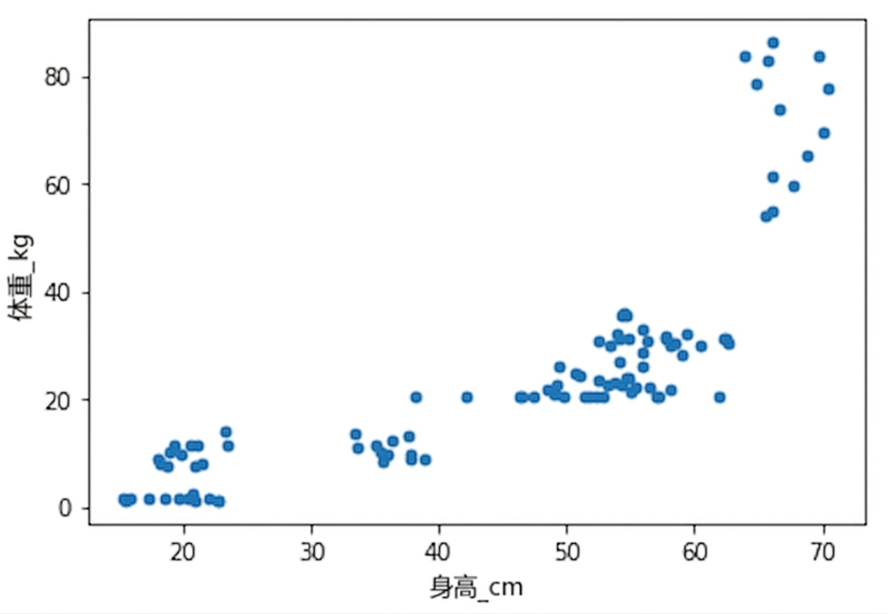
狗的体重与身高的散点图。身高越高，体重越重。存在一些聚类，可能对应不同品种。

图层叠加

dog_pack[dog_pack["sex"]=="F"]["height_cm"].hist()
dog_pack[dog_pack["sex"]=="M"]["height_cm"].hist()

plt.show()

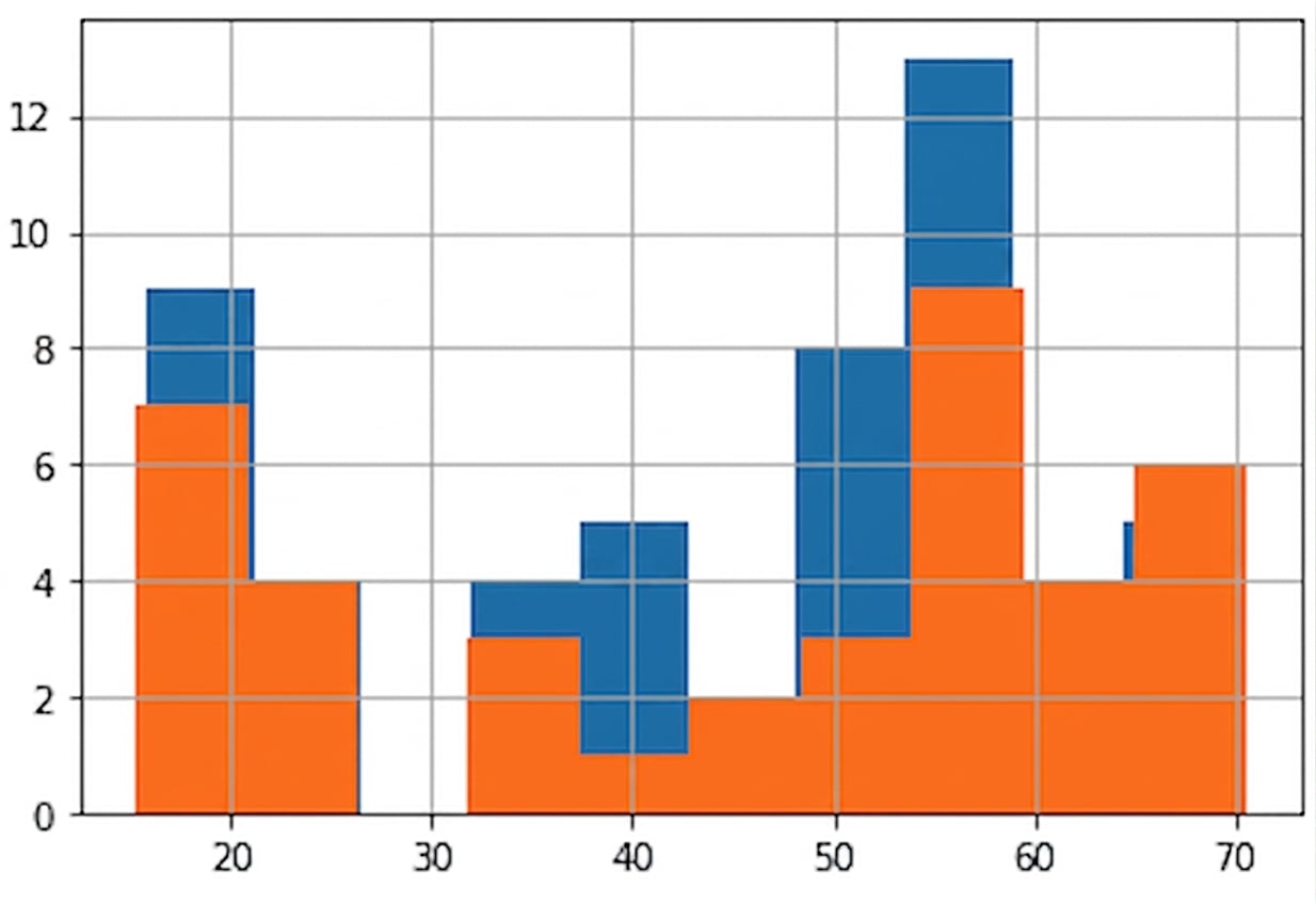
同一图中显示两组狗身高直方图。一组为蓝色，一组为橙色。橙色直方图覆盖蓝色，使细节难以分辨。

添加图例

dog_pack[dog_pack["sex"]=="F"]["height_cm"].hist()
dog_pack[dog_pack["sex"]=="M"]["height_cm"].hist()
plt.legend(["F", "M"])
plt.show()

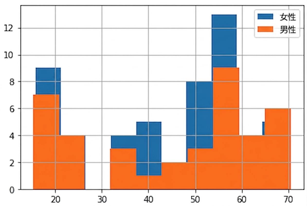
与上一页相同的两组直方图，但添加了图例。"F"（雌）为蓝色，"M"（雄）为橙色。仍然难以看清细节。

透明度

dog_pack[dog_pack["sex"]=="F"]["height_cm"].hist(alpha=0.7)
dog_pack[dog_pack["sex"]=="M"]["height_cm"].hist(alpha=0.7)
plt.legend(["F", "M"])
plt.show()

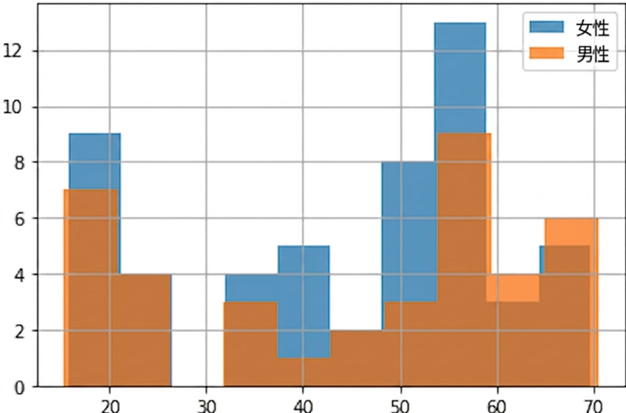
与上一页相同的两组直方图，但直方图已半透明。可见先前被遮挡的雌性柱子。仍略显杂乱。想要更美观的图，可学习 Seaborn 课程。

牛油果数据

print(avocados)

            date          type  year  avg_price         size     nb_sold
0     2015-12-27  conventional  2015       0.95        small  9626901.09
1     2015-12-20  conventional  2015       0.98        small  8710021.76
2     2015-12-13  conventional  2015       0.93        small  9855053.66
...          ...           ...   ...        ...          ...         ...
1011  2018-01-21       organic  2018       1.63  extra_large     1490.02
1012  2018-01-14       organic  2018       1.59  extra_large     1580.01
1013  2018-01-07       organic  2018       1.51  extra_large     1289.07

[1014 rows x 6 columns]

¡Vamos a practicar!

使用 pandas 进行数据处理