条形图

使用 ggplot2 进行数据可视化入门

Rick Scavetta

Founder, Scavetta Academy

条形图：分类 X 轴

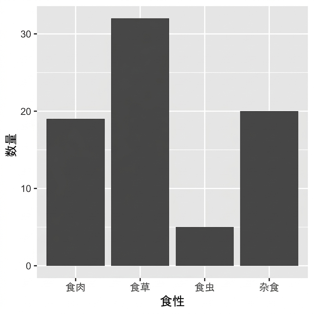
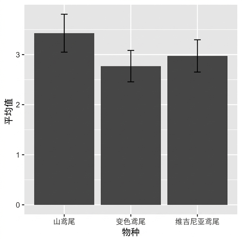
使用 geom_bar() 或 geom_col()

几何对象	统计	动作
`geom_bar()`	"count"	统计每个 x 位置的案例数
`geom_col()`	"identity"	绘制实际数值

之前的所有 position 均可用
两种类型
- 绝对计数
- 分布

条形图：分类 X 轴

使用 geom_bar() 或 geom_col()

几何对象	统计	动作
`geom_bar()`	"count"	统计每个 x 位置的案例数
`geom_col()`	"identity"	绘制实际数值

条形图：分类 X 轴

使用 geom_bar() 或 geom_col()

几何对象	统计	动作
`geom_bar()`	"count"	统计每个 x 位置的案例数
`geom_col()`	"identity"	绘制实际数值

之前的所有 position 均可用
两种类型
- 绝对计数
- 分布

哺乳动物的食性

str(sleep)

'data.frame':    76 obs. of  3 variables:
 $ vore : Factor w/ 4 levels "carni","herbi",..: 1 4 2 4 2 2 1 1 2 2 ...
 $ total: num  12.1 17 14.4 14.9 4 14.4 8.7 10.1 3 5.3 ...
 $ rem  : num  NA 1.8 2.4 2.3 0.7 2.2 1.4 2.9 NA 0.6 ...

条形图

ggplot(sleep, aes(vore)) + 
  geom_bar()

绘制分布而非绝对计数

# Calculate Descriptive Statistics:
iris %>% 
  select(Species, Sepal.Width) %>% 
  pivot_longer(!Species, names_to = "key", 
  values_to = "value") %>%
  group_by(Species) %>% 
  summarise(avg = mean(value), 
            stdev = sd(value))
   -> iris_summ_long

iris_summ_long

Species	avg	stdev
setosa	3.43	0.38
versicolor	2.77	0.31
virginica	2.97	0.32

绘制分布

ggplot(iris_summ_long, aes(x = Species, 
                           y = avg)) + 
  geom_col() +
  geom_errorbar(aes(ymin = avg - stdev, 
                    ymax = avg + stdev), 
                width = 0.1)

让我们来练习！

使用 ggplot2 进行数据可视化入门