修改美学属性

使用 ggplot2 进行数据可视化入门

Rick Scavetta

Founder, Scavetta Academy

位置(Positions)

重叠调整方式

  • identity
  • dodge
  • stack
  • fill
  • jitter
  • jitterdodge
  • nudge
使用 ggplot2 进行数据可视化入门

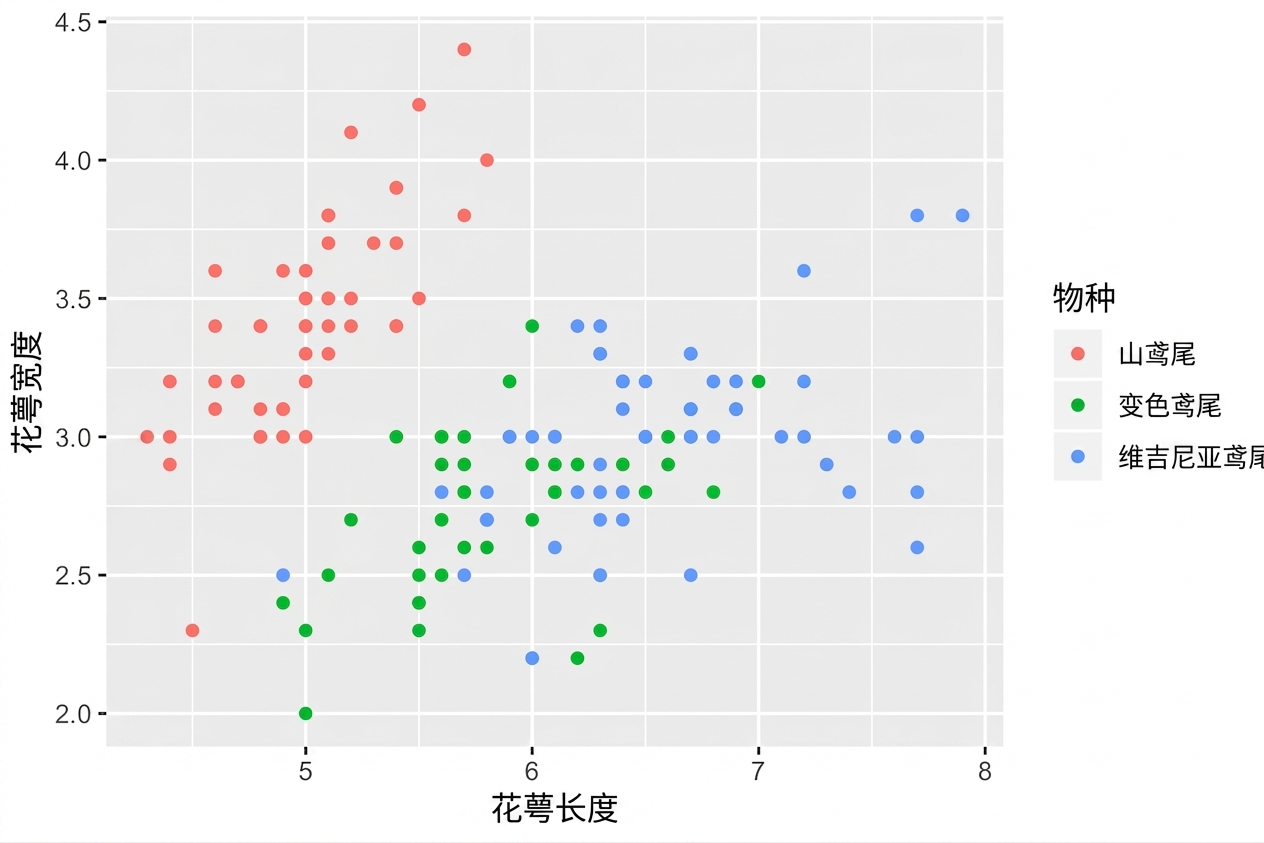
position = "identity"(默认)

ggplot(iris, aes(x = Sepal.Length, 
                 y = Sepal.Width, 
                 color = Species)) + 
  geom_point()

使用 ggplot2 进行数据可视化入门

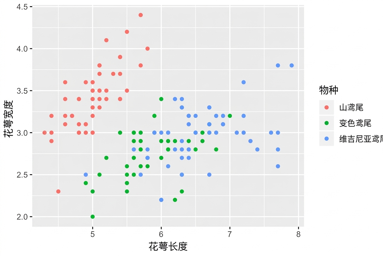
position = "identity"(默认)

ggplot(iris, aes(x = Sepal.Length, 
                 y = Sepal.Width, 
                 color = Species)) + 
  geom_point(position = "identity")

使用 ggplot2 进行数据可视化入门

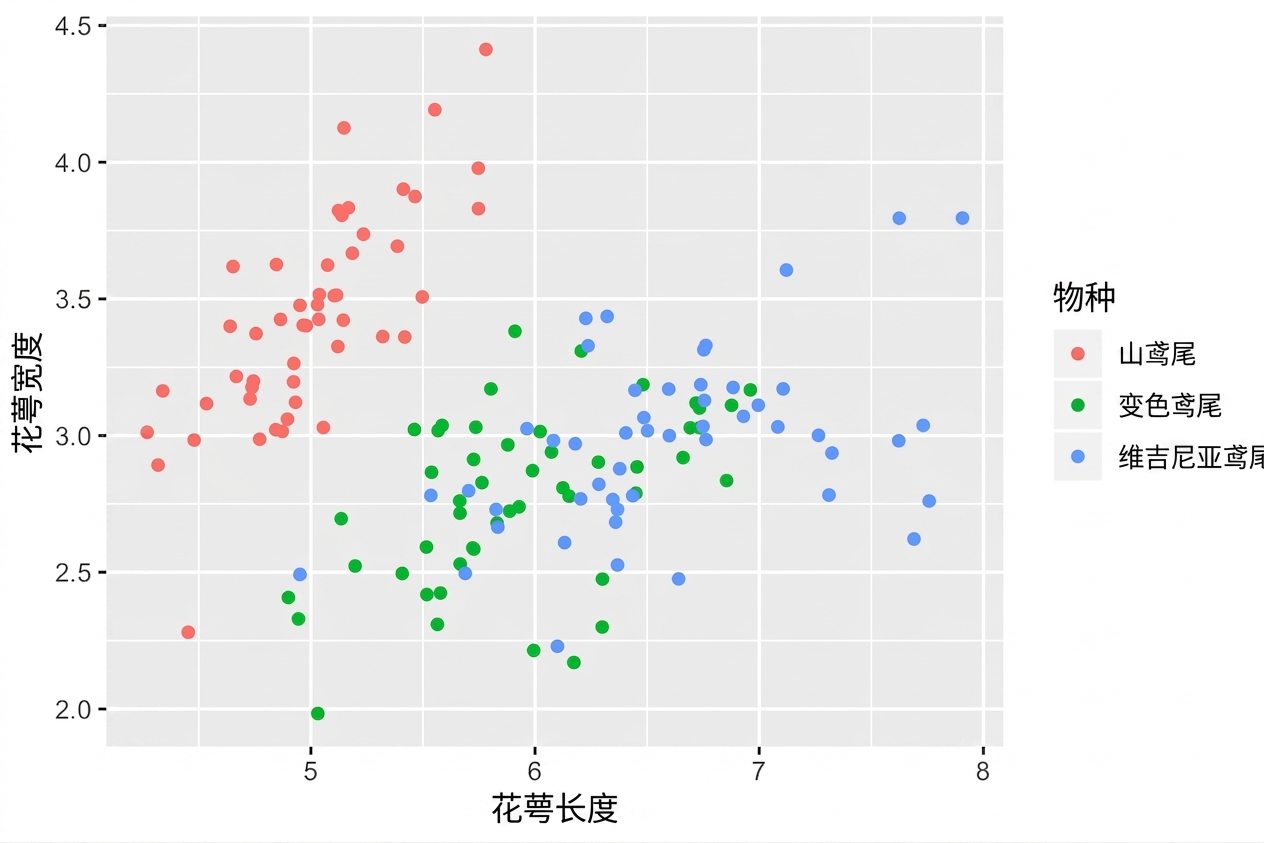
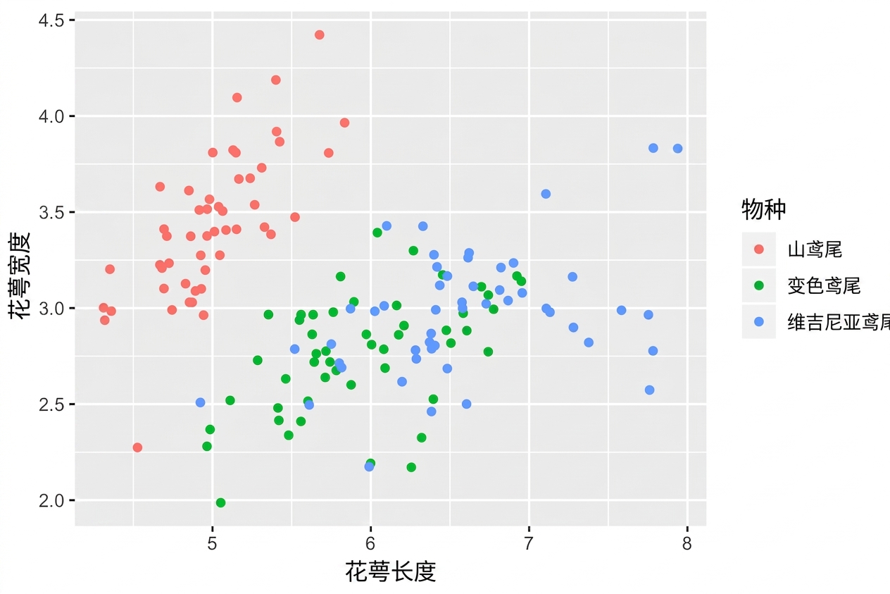
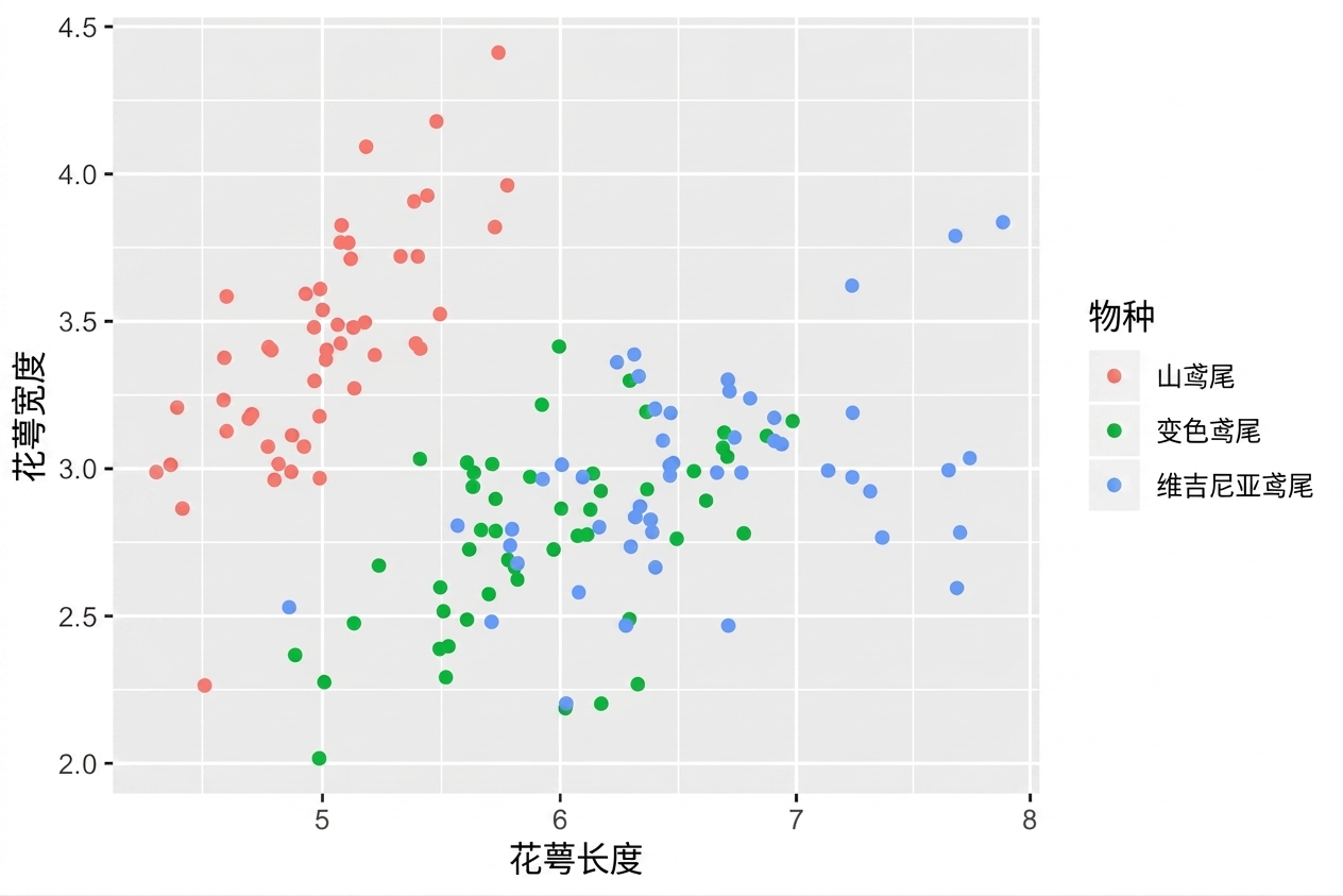
position = "jitter"

ggplot(iris, aes(x = Sepal.Length, 
                 y = Sepal.Width, 
                 color = Species)) + 
  geom_point(position = "jitter")

使用 ggplot2 进行数据可视化入门

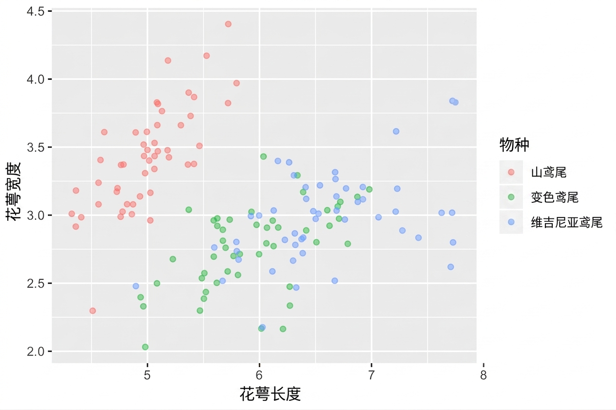
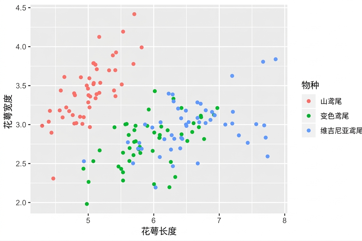
position_jitter()

posn_j <- position_jitter(0.1)

ggplot(iris, aes(x = Sepal.Length, 
                 y = Sepal.Width, 
                 col = Species)) +
  geom_point(position = posn_j)

使用 ggplot2 进行数据可视化入门

position_jitter()

posn_j <- position_jitter(0.1, 
                          seed = 136)

ggplot(iris, aes(x = Sepal.Length, 
                 y = Sepal.Width, 
                 color = Species)) + 
  geom_point(position = posn_j)
  • 设置位置参数
  • 各图与图层保持一致性

使用 ggplot2 进行数据可视化入门

刻度函数(Scale)

  • scale_x_*()
  • scale_y_*()
  • scale_color_*()
    • 也可用 scale_colour_*()
  • scale_fill_*()
  • scale_shape_*()
  • scale_linetype_*()
  • scale_size_*()
使用 ggplot2 进行数据可视化入门

刻度函数(Scale)

  • scale_x_continuous()
  • scale_y_*()
  • scale_color_discrete()
    • scale_colour_*()
  • scale_fill_*()
  • scale_shape_*()
  • scale_linetype_*()
  • scale_size_*()
使用 ggplot2 进行数据可视化入门

scale_*_*()

ggplot(iris, aes(x = Sepal.Length, 
                 y = Sepal.Width, 
                 color = Species)) + 
  geom_point(position = "jitter") +
  scale_x_continuous("Sepal Length") +
  scale_color_discrete("Species")

使用 ggplot2 进行数据可视化入门

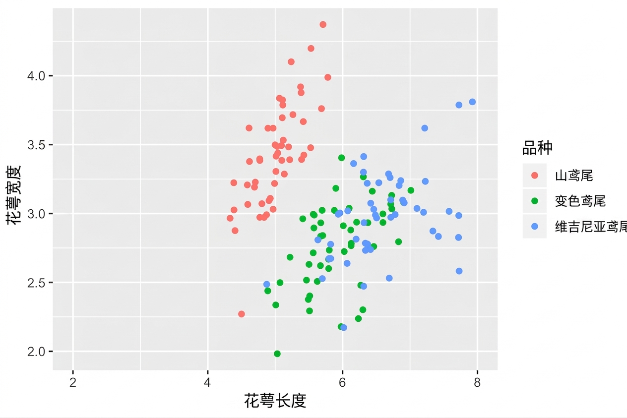
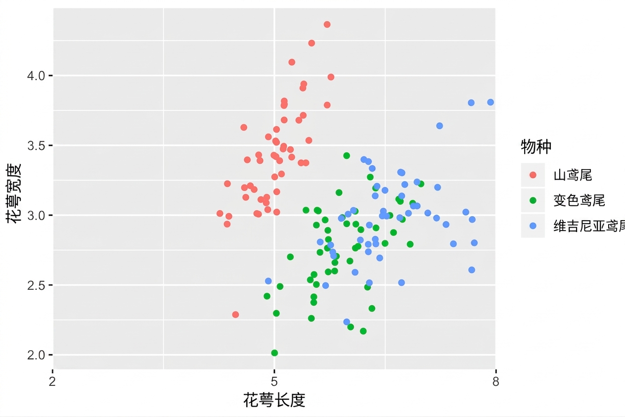
limits 参数

ggplot(iris, aes(x = Sepal.Length, 
                  y = Sepal.Width, 
                 color = Species)) + 
  geom_point(position = "jitter") +
  scale_x_continuous("Sepal Length", 
                     limits = c(2,8)) +
  scale_color_discrete("Species")

使用 ggplot2 进行数据可视化入门

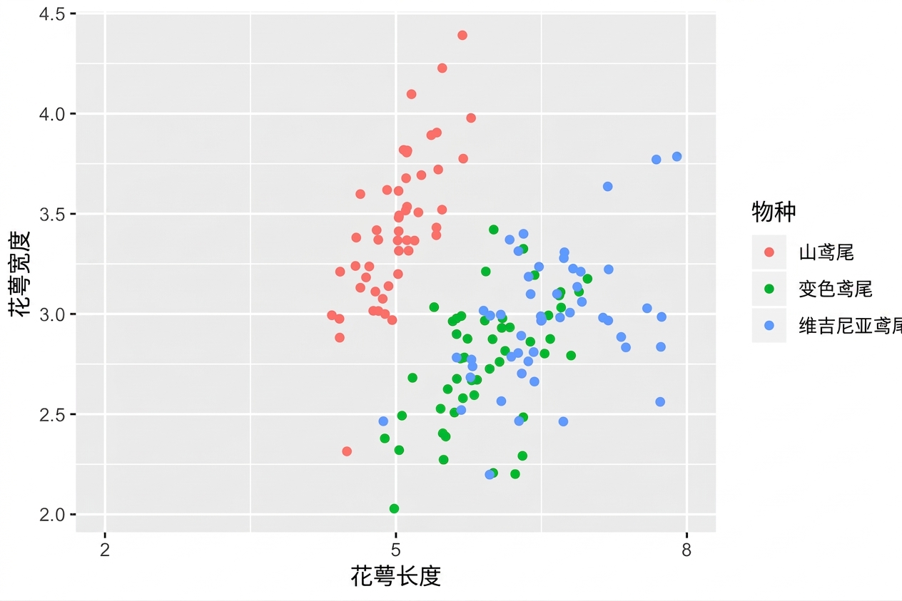
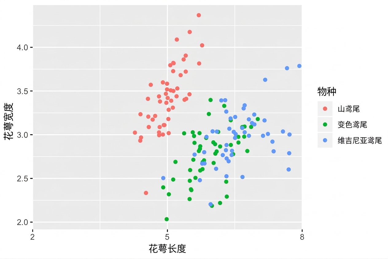
breaks 参数

ggplot(iris, aes(x = Sepal.Length, 
                  y = Sepal.Width, 
                 color = Species)) + 
  geom_point(position = "jitter") +
  scale_x_continuous("Sepal Length", 
                     limits = c(2, 8), 
                     breaks = seq(2, 8, 3)) +
  scale_color_discrete("Species")

使用 ggplot2 进行数据可视化入门

expand 参数

ggplot(iris, aes(x = Sepal.Length, 
                  y = Sepal.Width, 
                 color = Species)) + 
  geom_point(position = "jitter") +
  scale_x_continuous("Sepal Length", 
                     limits = c(2, 8), 
                     breaks = seq(2, 8, 3),
                     expand = c(0, 0)) +
  scale_color_discrete("Species")

使用 ggplot2 进行数据可视化入门

labels 参数

ggplot(iris, aes(x = Sepal.Length, 
                  y = Sepal.Width, 
                 color = Species)) + 
  geom_point(position = "jitter") +
  scale_x_continuous("Sepal Length", 
                     limits = c(2, 8), 
                     breaks = seq(2, 8, 3),
                     expand = c(0, 0), 
                     labels = c("Setosa", 
                               "Versicolor", 
                               "Virginica")) +
  scale_color_discrete("Species")

使用 ggplot2 进行数据可视化入门

labs()

ggplot(iris, aes(x = Sepal.Length, 
                 y = Sepal.Width, 
                 color = Species)) +
  geom_point(position = "jitter") +
  labs(x = "Sepal Length", 
       y = "Sepal Width", 
       color = "Species")

使用 ggplot2 进行数据可视化入门

让我们试试吧!

使用 ggplot2 进行数据可视化入门

Preparing Video For Download...