散点图

使用 ggplot2 进行数据可视化入门

Rick Scavetta

Founder, Scavetta Academy

48 种几何图层

geom_*
abline contour dotplot jitter pointrange ribbon spoke
area count errorbar label polygon rug step
bar crossbar errorbarh line qq segment text
bin2d curve freqpoly linerange qq_line sf tile
blank density hex map quantile sf_label violin
boxplot density2d histogram path raster sf_text vline
col density_2d hline point rect smooth
使用 ggplot2 进行数据可视化入门

常见图类型

图类型 可用 Geom
散点图 points, jitter, abline, smooth, count
使用 ggplot2 进行数据可视化入门

散点图

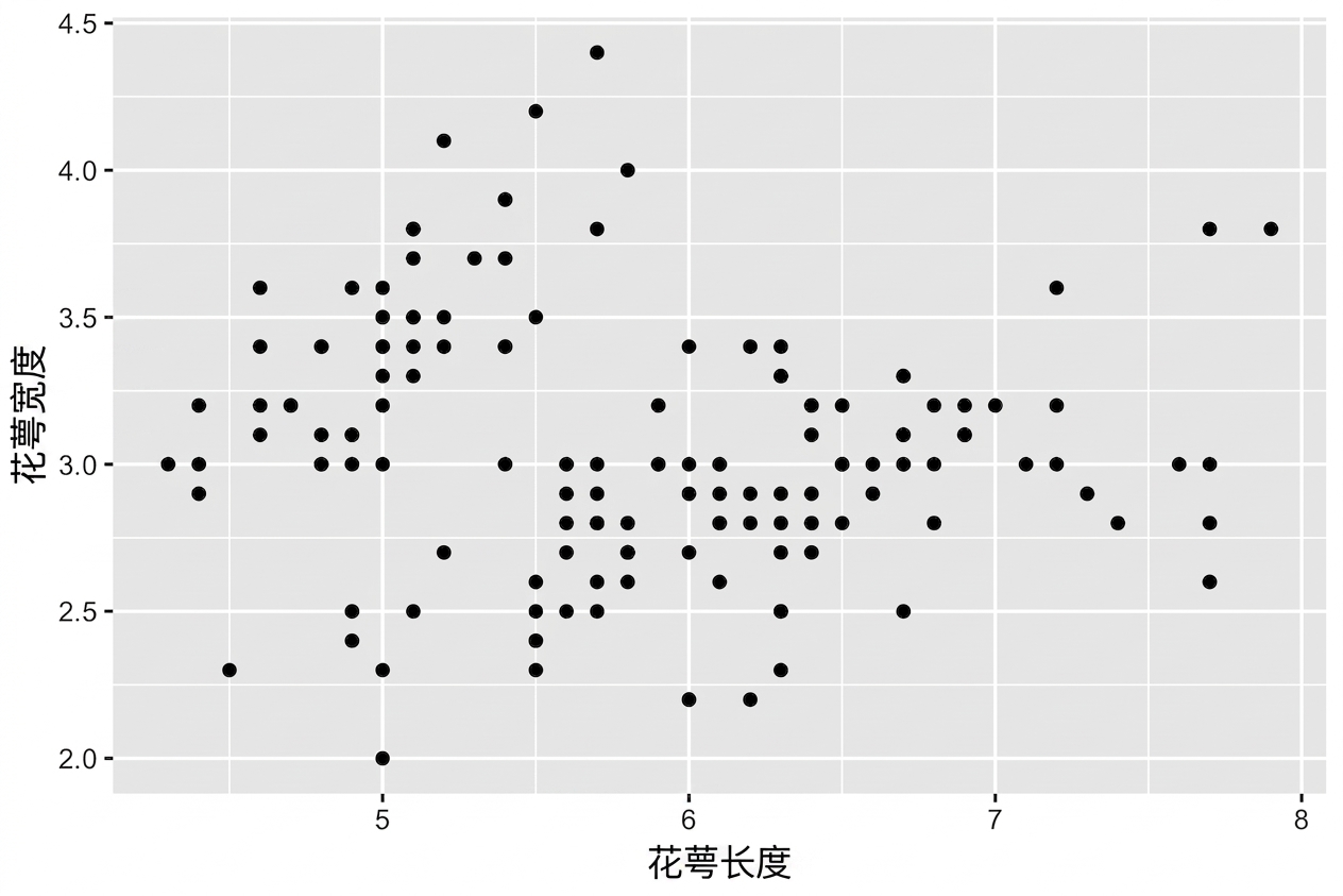
  • 每个几何图层可接受特定美学映射,如 geom_point():
必需
x,y
ggplot(iris, aes(x = Sepal.Length, 
                 y = Sepal.Width)) + 
  geom_point()
使用 ggplot2 进行数据可视化入门

散点图

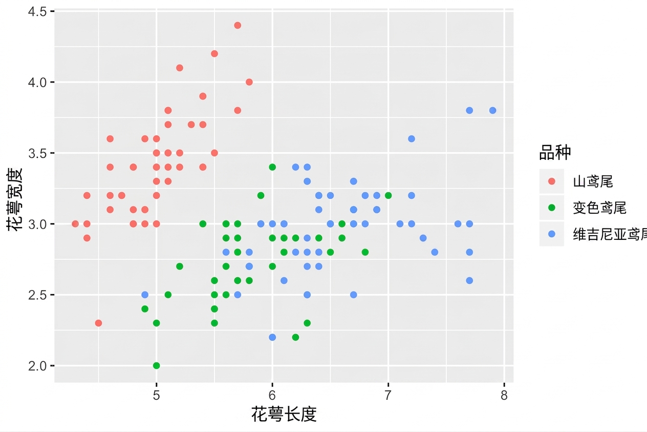
  • 每个几何图层可接受特定美学映射,如 geom_point():
必需 可选
x,y alpha, color, fill, shape, size, stroke
ggplot(iris, aes(x = Sepal.Length, 
                 y = Sepal.Width,
                 col = Species)) + 
  geom_point()
使用 ggplot2 进行数据可视化入门

几何图层专属映射

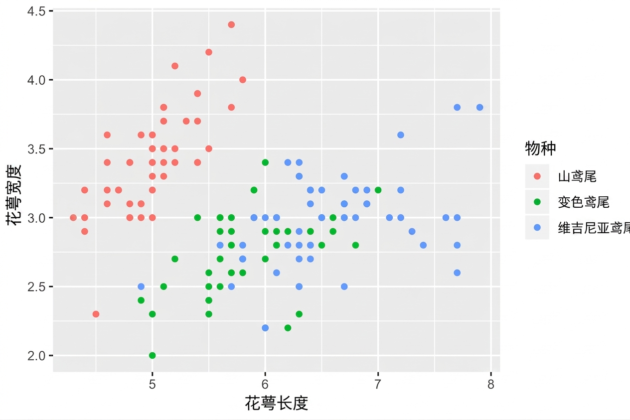
# 这两段代码生成相同的图!
ggplot(iris, aes(x = Sepal.Length, y = Sepal.Width, col = Species)) + 
  geom_point()

ggplot(iris, aes(x = Sepal.Length, y = Sepal.Width)) + 
  geom_point(aes(col = Species))

可分别控制每一层的美学映射:
使用 ggplot2 进行数据可视化入门
head(iris, 3) # 原始数据
Species Sepal.Length Sepal.Width Petal.Length Petal.Width
1  setosa          5.1         3.5          1.4         0.2
2  setosa          4.9         3.0          1.4         0.2
3  setosa          4.7         3.2          1.3         0.2
iris %>%
  group_by(Species) %>% 
  summarise_all(mean) -> iris.summary

iris.summary # 汇总统计
# A tibble: 3 x 5
  Species    Sepal.Length Sepal.Width Petal.Length Petal.Width
  <fct>             <dbl>       <dbl>        <dbl>       <dbl>
1 setosa             5.01        3.43         1.46       0.246
2 versicolor         5.94        2.77         4.26       1.33 
3 virginica          6.59        2.97         5.55       2.03
使用 ggplot2 进行数据可视化入门
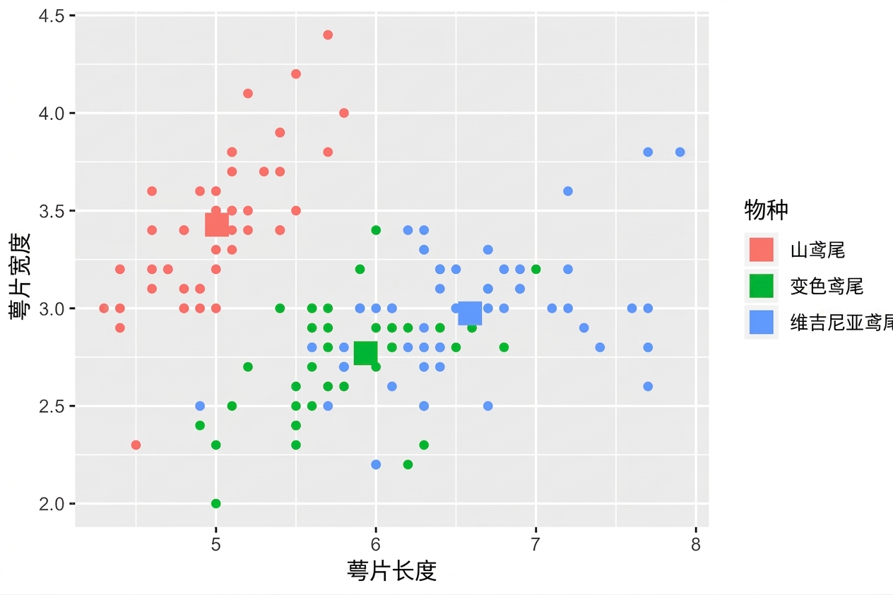
ggplot(iris, aes(x = Sepal.Length, y = Sepal.Width, col = Species)) +
  # 从 ggplot() 继承数据和映射 
  geom_point() + 
  # 使用不同数据,但继承映射
  geom_point(data = iris.summary, shape = 15, size = 5)
使用 ggplot2 进行数据可视化入门

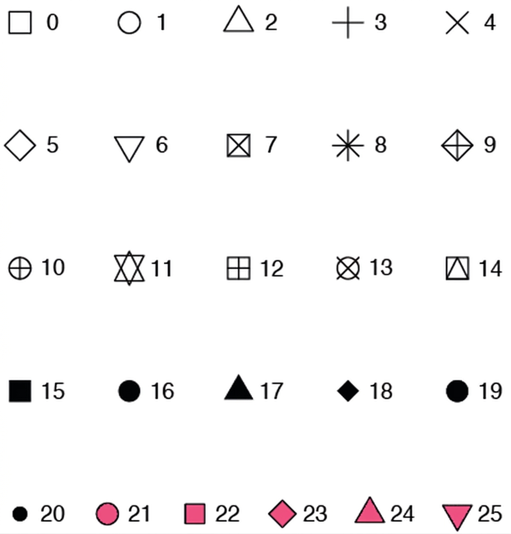
形状属性取值

使用 ggplot2 进行数据可视化入门

示例

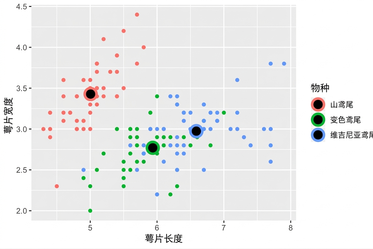
ggplot(iris, aes(x = Sepal.Length, y = Sepal.Width, col = Species)) + 
  geom_point() +
  geom_point(data = iris.summary, shape = 21, size = 5, 
             fill = "black", stroke = 2)
使用 ggplot2 进行数据可视化入门

ggplot2 的即时统计

  • 统计层见第二门课程。
  • 注意:避免只绘制均值而无离散度指标,如标准差。

使用 ggplot2 进行数据可视化入门

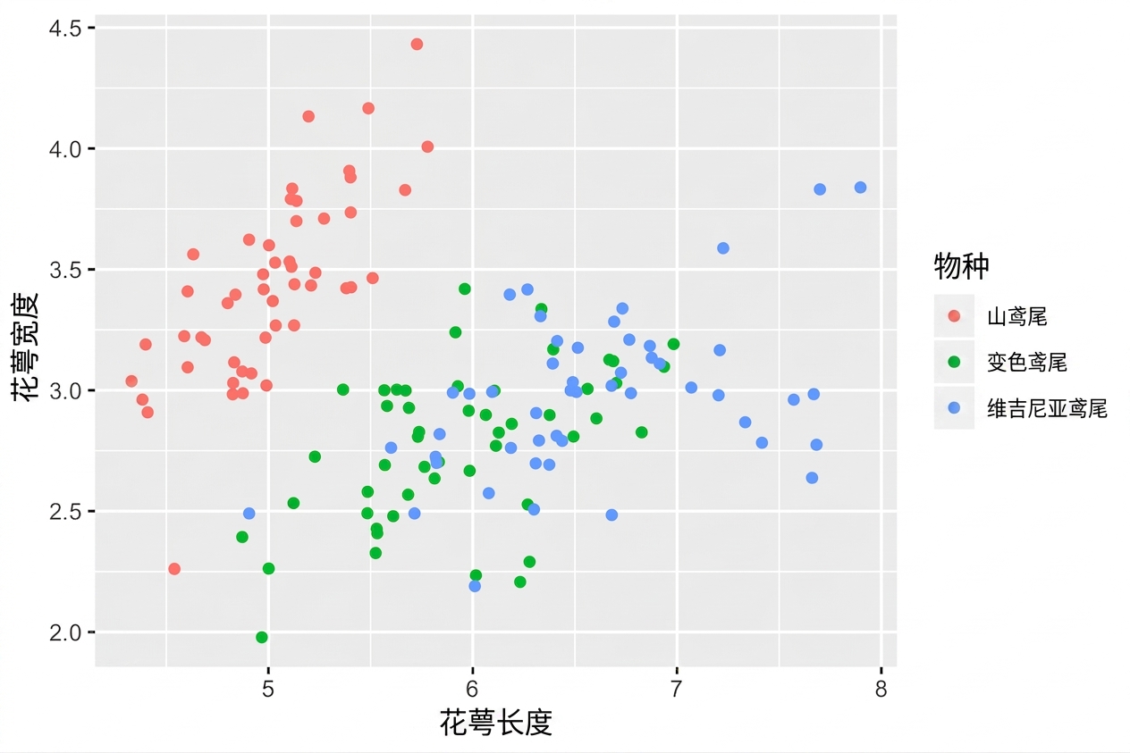
position = "jitter"

ggplot(iris, aes(x = Sepal.Length, y = Sepal.Width, col = Species)) + 
  geom_point(position = "jitter")
使用 ggplot2 进行数据可视化入门

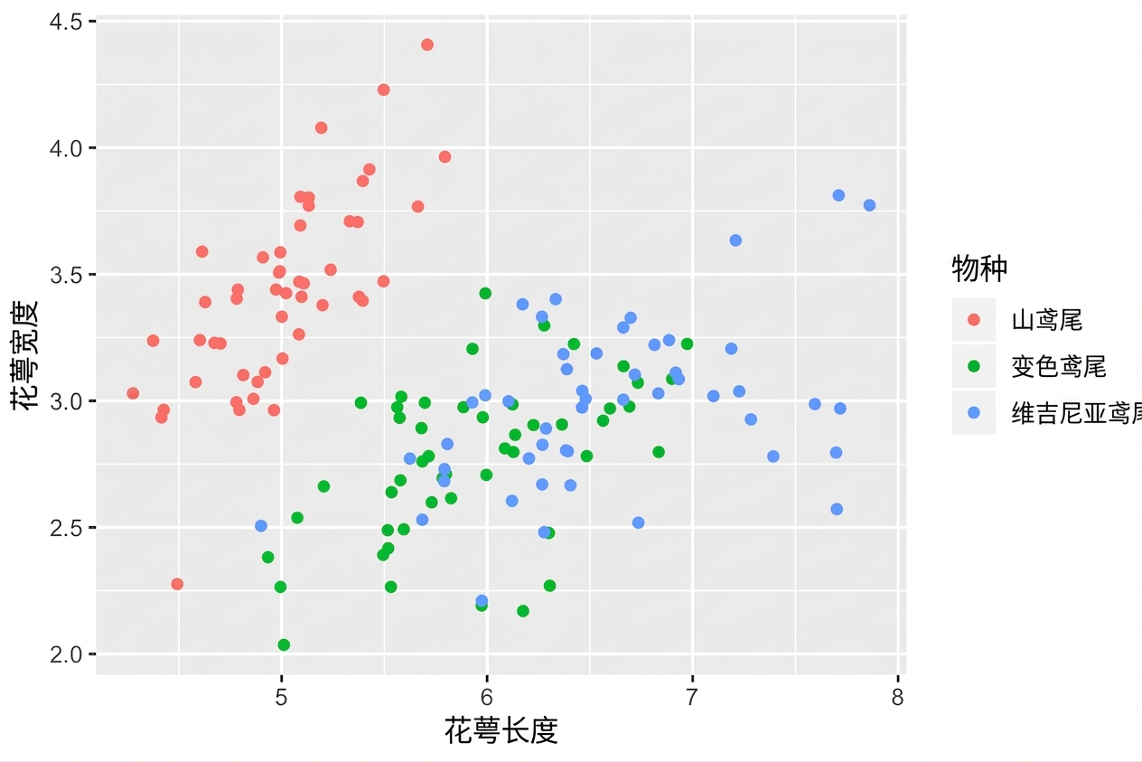
geom_jitter()

geom_point(position = "jitter") 的简写

ggplot(iris, aes(x = Sepal.Length, y = Sepal.Width, col = Species)) + 
  geom_jitter()
使用 ggplot2 进行数据可视化入门

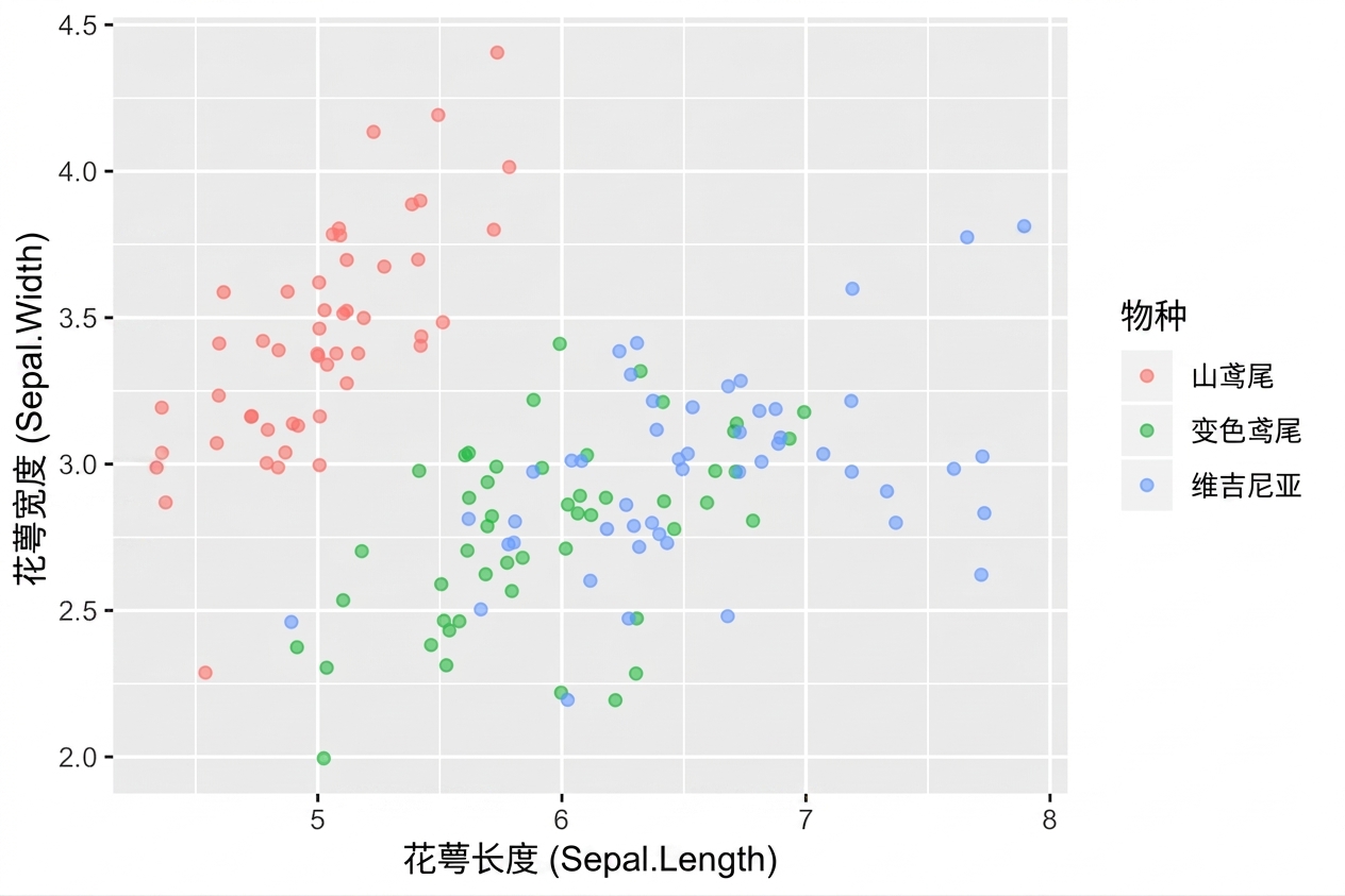
别忘了调透明度 alpha

  • 需要时将抖动与透明度叠加
ggplot(iris, aes(x = Sepal.Length, y = Sepal.Width, col = Species)) + 
  geom_jitter(alpha = 0.6)
使用 ggplot2 进行数据可视化入门

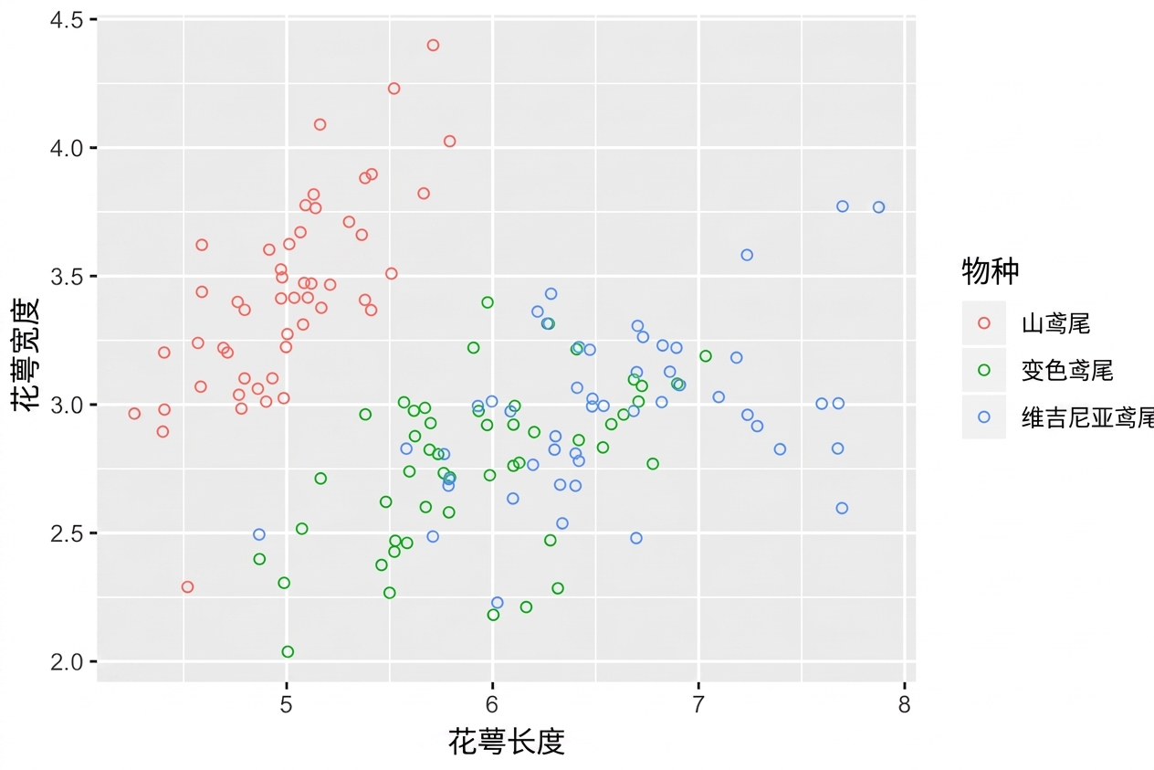
空心圆也有用

  • shape = 1 是空心圆。
  • 无需再用透明度。
ggplot(iris, aes(x = Sepal.Length, y = Sepal.Width, col = Species)) + 
  geom_jitter(shape = 1)
使用 ggplot2 进行数据可视化入门

开始练习吧!

使用 ggplot2 进行数据可视化入门

Preparing Video For Download...