变量变换

R 中的回归入门

Richie Cotton

Data Evangelist at DataCamp

鲈鱼数据集

library(dplyr)

perch <- fish %>%
  filter(species == "Perch")
species mass_g length_cm
Perch 5.9 7.5
Perch 32.0 12.5
Perch 40.0 13.8
Perch 51.5 15.0
Perch 70.0 15.7
... ... ...
R 中的回归入门

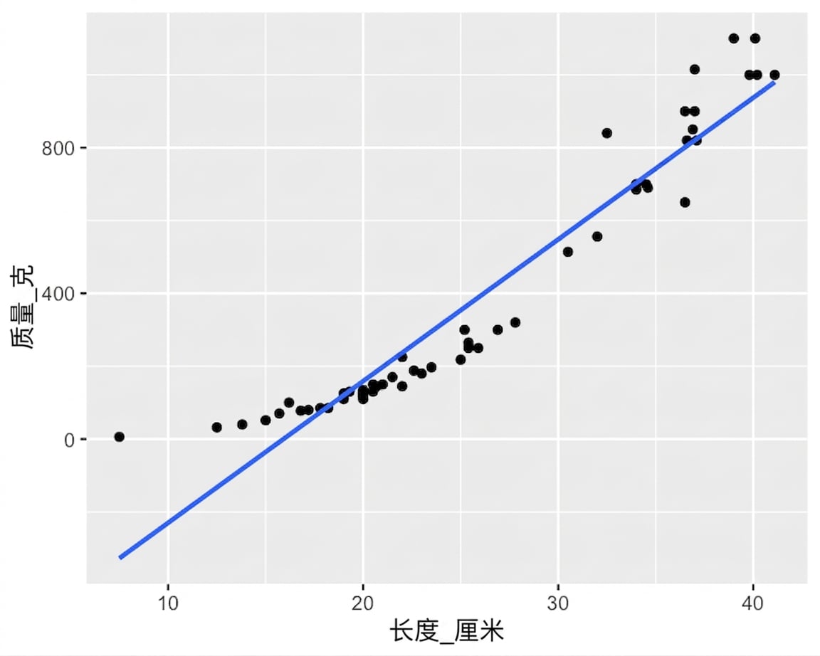
不是线性关系

ggplot(perch, aes(length_cm, mass_g)) +
  geom_point() +
  geom_smooth(method = "lm", se = FALSE)

鲈鱼质量与长度的散点图及趋势线。鲈鱼变长时,质量增长快于线性,形成向上的弧线。

R 中的回归入门

鲷鱼 vs. 鲈鱼

一些鲷鱼在游动。鲷鱼很扁。

一些鲈鱼在游动。鲈鱼较为圆胖。

R 中的回归入门

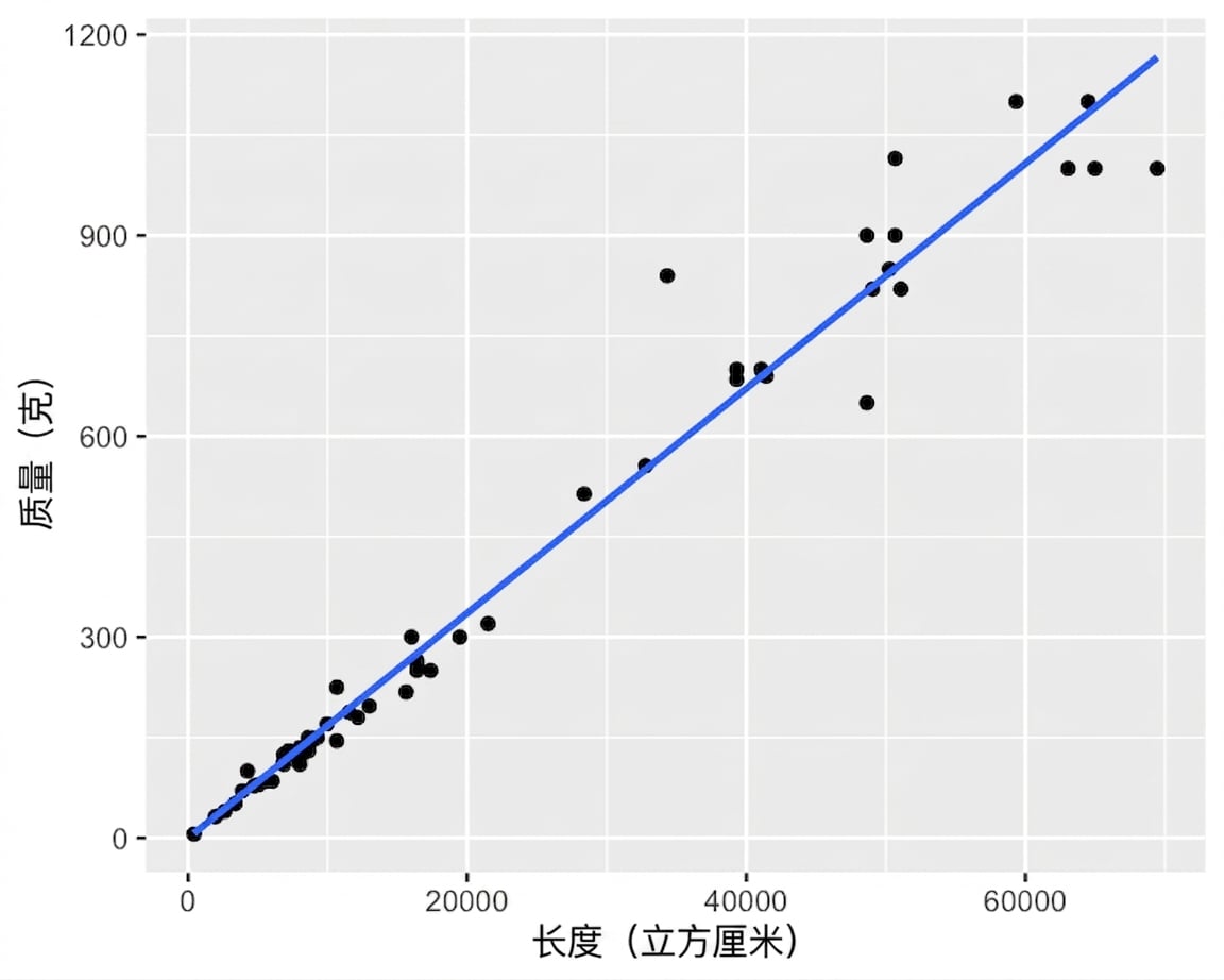
绘制 质量 vs 长度立方

ggplot(perch, aes(length_cm ^ 3, mass_g)) +
  geom_point() +
  geom_smooth(method = "lm", se = FALSE)

鲈鱼质量与长度的立方的散点图及趋势线。变换后,大多数点靠近趋势线。

R 中的回归入门

建模:质量 vs 长度立方

mdl_perch <- lm(mass_g ~ I(length_cm ^ 3), data = perch)
Call:
lm(formula = mass_g ~ I(length_cm^3), data = perch)

Coefficients:
   (Intercept)  I(length_cm^3)  
       -0.1175          0.0168
R 中的回归入门

预测:质量 vs 长度立方

explanatory_data <- tibble(
  length_cm = seq(10, 40, 5)
)
prediction_data <- explanatory_data %>%
  mutate(
    mass_g = predict(mdl_perch, explanatory_data)
  )
# A tibble: 7 x 2
  length_cm mass_g
      <dbl>  <dbl>
1        10   16.7
2        15   56.6
3        20  134. 
4        25  262. 
5        30  453. 
6        35  720. 
7        40 1075.
R 中的回归入门

绘制 质量 vs 长度立方

ggplot(perch, aes(length_cm ^ 3, mass_g)) +
  geom_point() +
  geom_smooth(method = "lm", se = FALSE) +
  geom_point(data = prediction_data, color = "blue")
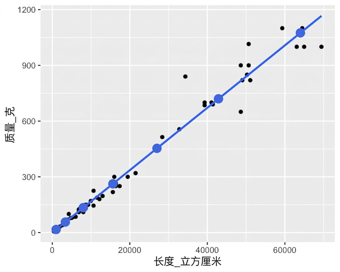
质量与长度立方的散点图和趋势线,并标注由 predict() 计算的点。这些点完全沿着趋势线。

ggplot(perch, aes(length_cm, mass_g)) +
  geom_point() +
  geom_smooth(method = "lm", se = FALSE) +
  geom_point(data = prediction_data, color = "blue")
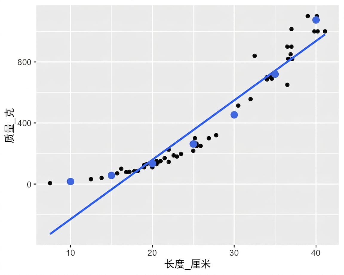
质量与长度的散点图和趋势线,并标注由 predict() 计算的点。这些点不沿趋势线,但沿着数据点的弯曲形状。

R 中的回归入门

Facebook 广告数据集

广告如何运作

  1. 付费给 Facebook 投放广告。
  2. 人们看到广告("展示量")。
  3. 部分看到的人会点击。


  • 936 行
  • 每行代表 1 个广告
spent_usd n_impressions n_clicks
1.43 7350 1
1.82 17861 2
1.25 4259 1
1.29 4133 1
4.77 15615 3
... ... ...
R 中的回归入门

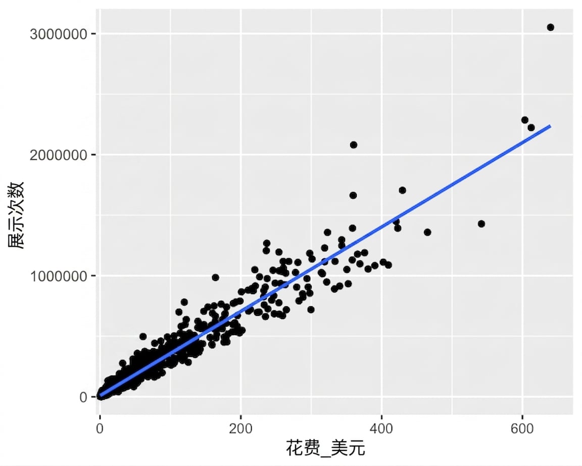
图太挤

ggplot(
  ad_conversion, 
  aes(spent_usd, n_impressions)
) +
  geom_point() +
  geom_smooth(method = "lm", se = FALSE)

展示量与广告花费的散点图及趋势线。多数点挤在图的左下角。

R 中的回归入门

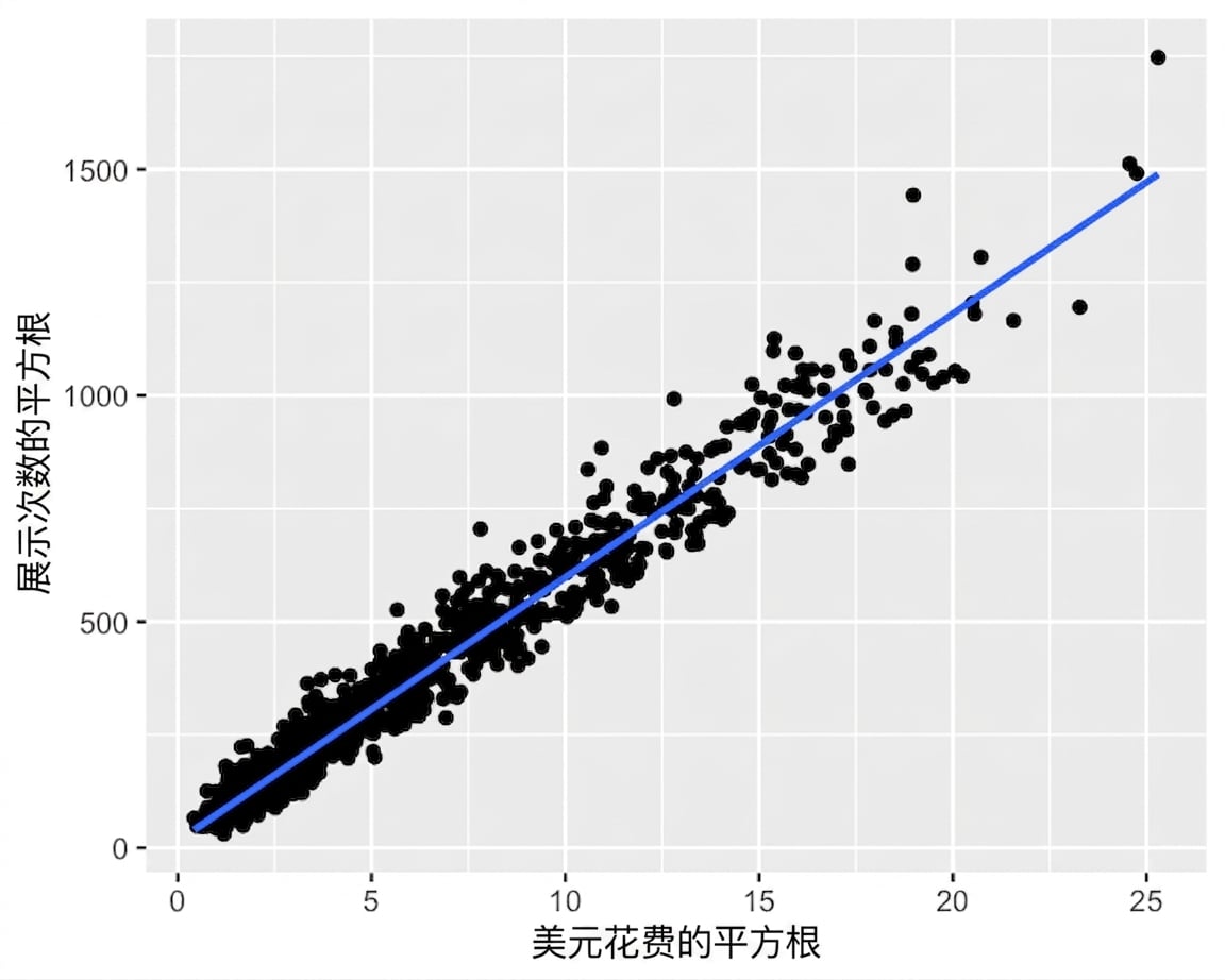
平方根 vs 平方根

ggplot(
  ad_conversion, 
  aes(sqrt(spent_usd), sqrt(n_impressions))
) +
  geom_point() +
  geom_smooth(method = "lm", se = FALSE)

展示量平方根与花费平方根的散点图及趋势线。现在点在图中分布更均匀。

R 中的回归入门

建模与预测

mdl_ad <- lm(
  sqrt(n_impressions) ~ sqrt(spent_usd), 
  data = ad_conversion
)
explanatory_data <- tibble(
  spent_usd = seq(0, 600, 100)
)
prediction_data <- explanatory_data %>% 
  mutate(
    sqrt_n_impressions = predict(
      mdl_ad, explanatory_data
    ),
    n_impressions = sqrt_n_impressions ^ 2
  )
# A tibble: 7 x 3
  spent_usd sqrt_n_impressions n_impressions
      <dbl>              <dbl>         <dbl>
1         0               15.3          235.
2       100              598.        357289.
3       200              839.        703890.
4       300             1024.       1048771.
5       400             1180.       1392762.
6       500             1318.       1736184.
7       600             1442.       2079202.
R 中的回归入门

开始练习吧!

R 中的回归入门

Preparing Video For Download...