预测与优势比

R 中的回归入门

Richie Cotton

Data Evangelist at DataCamp

ggplot 预测

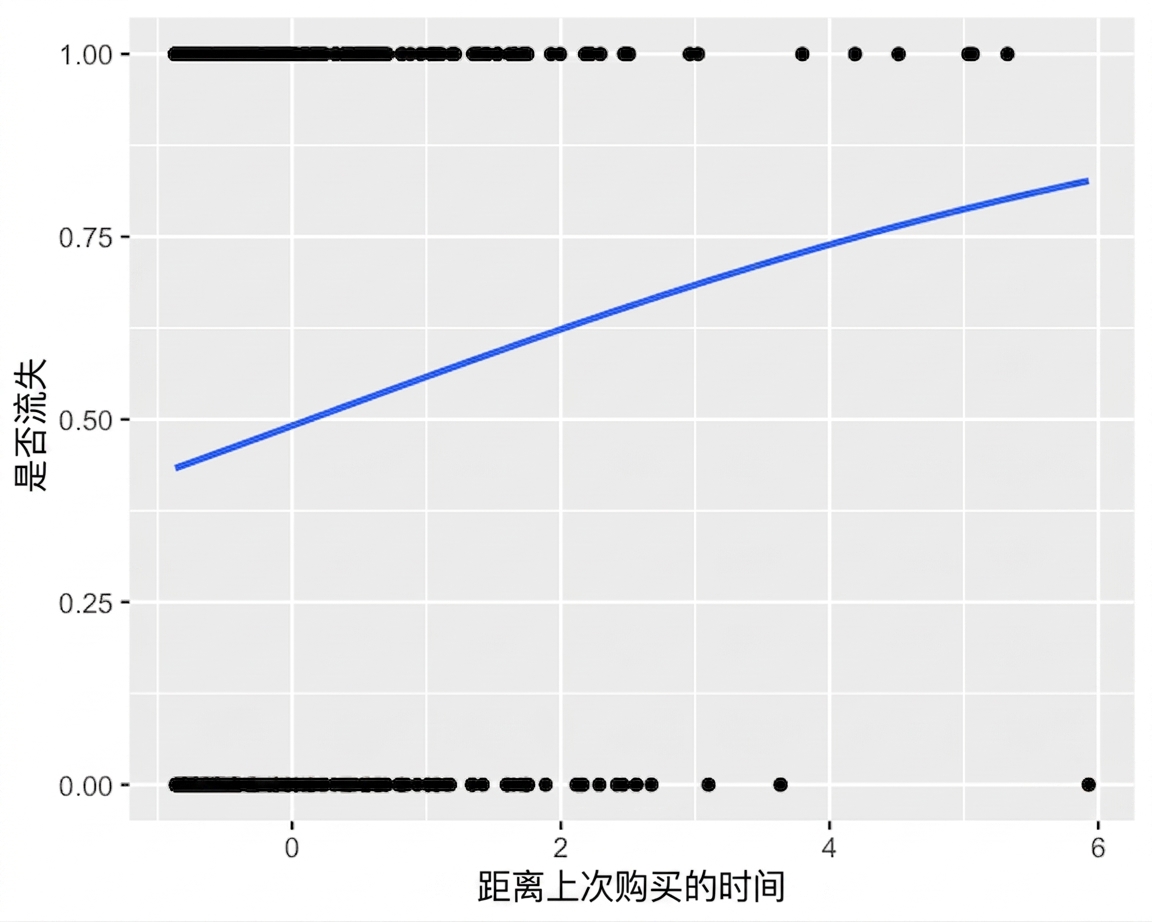
plt_churn_vs_recency_base <- ggplot(
  churn, 
  aes(time_since_last_purchase, has_churned)
) +
  geom_point() +
  geom_smooth(
    method = "glm", 
    se = FALSE, 
    method.args = list(family = binomial)
  )

流失与上次购买时间的散点图，带逻辑回归趋势线。

进行预测

mdl_recency <- glm(
  has_churned ~ time_since_last_purchase, data = churn, family = "binomial"
)

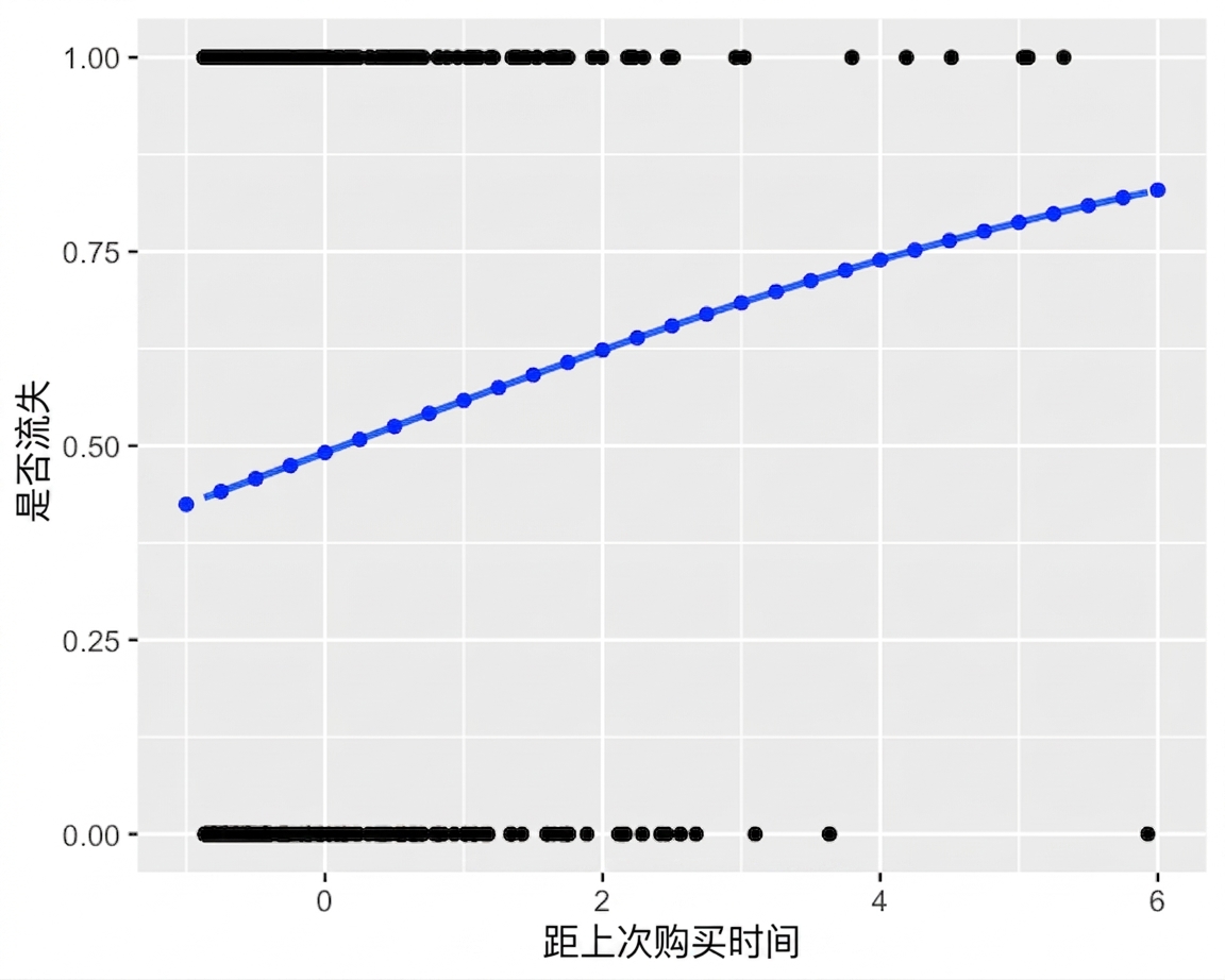
explanatory_data <- tibble(
  time_since_last_purchase = seq(-1, 6, 0.25)
)

prediction_data <- explanatory_data %>% 
  mutate(
    has_churned = predict(mdl_recency, explanatory_data, type = "response")
  )

添加点预测

plt_churn_vs_recency_base +
  geom_point(
    data = prediction_data, 
    color = "blue"
  )

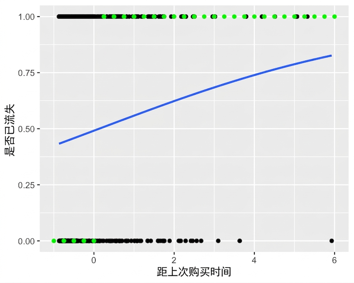
流失与上次购买时间的散点图，带逻辑回归趋势线。图中标注 predict() 的结果，与趋势线完全一致。

获取最可能结果

prediction_data <- explanatory_data %>% 
  mutate(
    has_churned = predict(mdl_recency, explanatory_data, type = "response"),
    most_likely_outcome = round(has_churned)
  )

可视化最可能结果

plt_churn_vs_recency_base +
  geom_point(
    aes(y = most_likely_outcome),
    data = prediction_data,
    color = "green"
  )

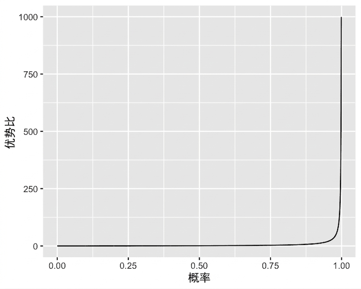
流失与上次购买时间的散点图，带逻辑回归趋势线。图中标注最可能结果：上次购买时间短时，最可能为不流失；时间长时，最可能为流失。

优势比（Odds ratio）

"优势比"是事件发生的概率除以不发生的概率。

$$ odds\_ratio = \frac{probability}{(1 - probability)} $$

$$ odds\_ratio = \frac{0.25}{(1 - 0.25)} = \frac{1}{3} $$

优势比与概率的折线图。概率趋近于1时，曲线渐近趋于无穷大。

计算优势比

prediction_data <- explanatory_data %>%
  mutate(
    has_churned = predict(mdl_recency, explanatory_data, type = "response"),
    most_likely_response = round(has_churned),
    odds_ratio = has_churned / (1 - has_churned)
  )

可视化优势比

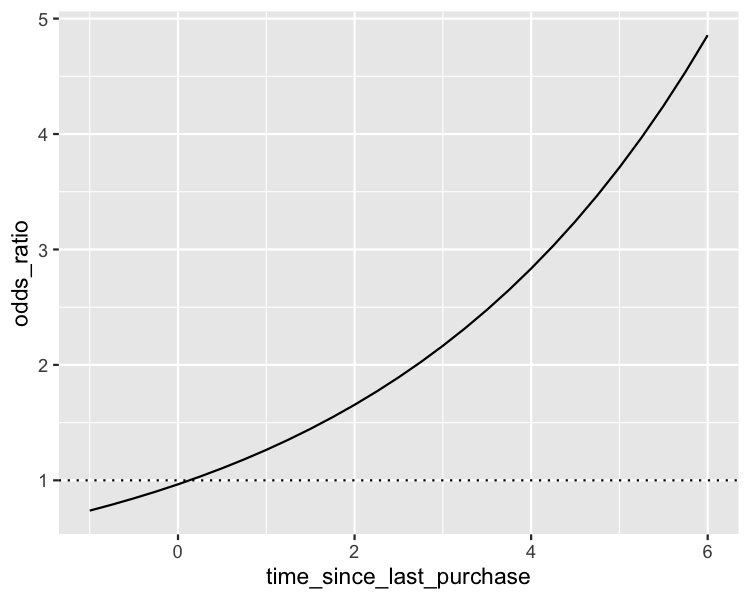
ggplot(
  prediction_data, 
  aes(time_since_last_purchase, odds_ratio)
) +
  geom_line() +
  geom_hline(yintercept = 1, linetype = "dotted")

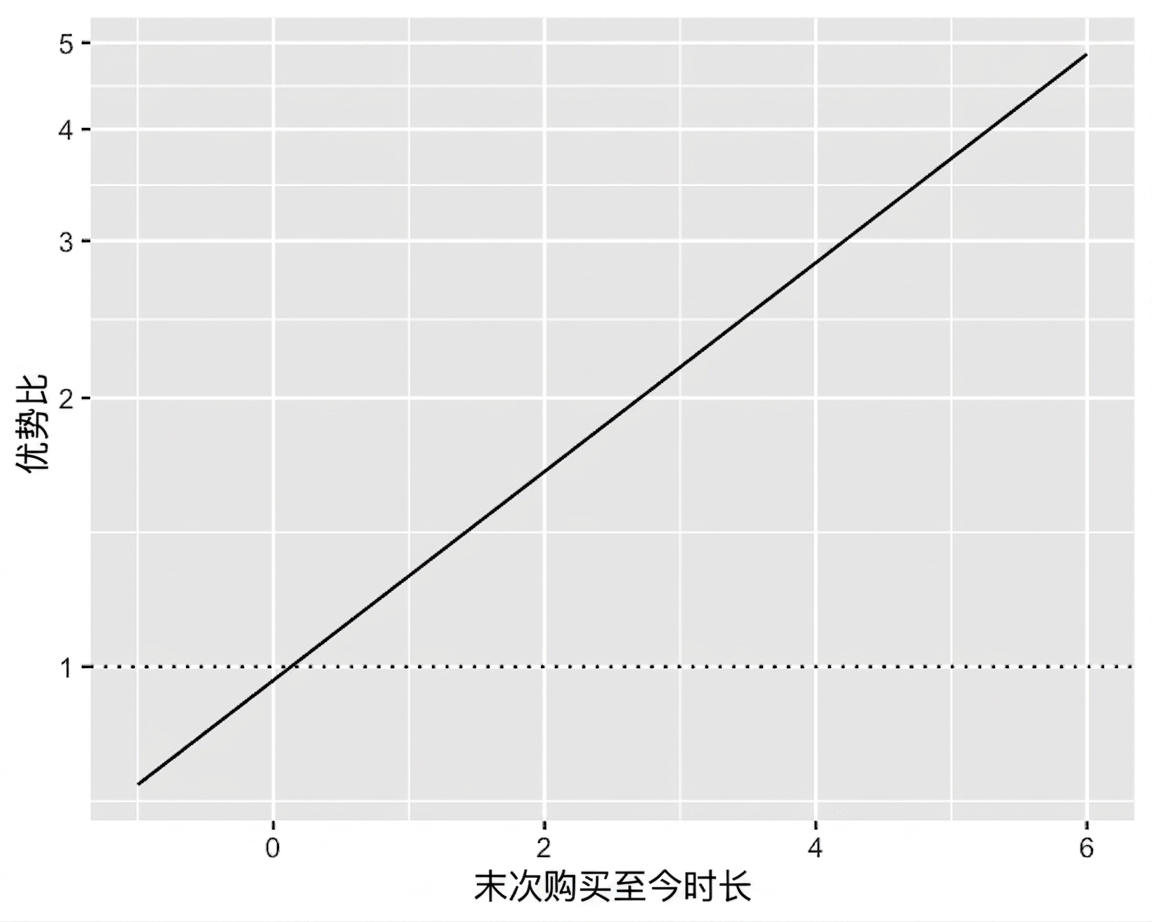
优势比与上次购买时间的折线图，含优势比=1的参考线。上次购买时间短时，最可能结果为不流失；时间越长，流失的优势比上升，最高约为不流失的5倍。

可视化对数优势比

ggplot(
  prediction_data, 
  aes(time_since_last_purchase, odds_ratio)
) +
  geom_line() +
  geom_hline(yintercept = 1, linetype = "dotted") +
  scale_y_log10()

优势比与上次购买时间的折线图，含优势比=1的参考线。y轴为对数刻度，使曲线近似线性。

计算对数优势比

prediction_data <- explanatory_data %>%
  mutate(
    has_churned = predict(mdl_recency, explanatory_data, type = "response"),
    most_likely_response = round(has_churned),
    odds_ratio = has_churned / (1 - has_churned),
    log_odds_ratio = log(odds_ratio),
    log_odds_ratio2 = predict(mdl_recency, explanatory_data)
  )

汇总所有预测

tm_snc_lst_prch	has_churned	most_lkly_rspns	odds_ratio	log_odds_ratio	log_odds_ratio2
0	0.491	0	0.966	-0.035	-0.035
2	0.623	1	1.654	0.503	0.503
4	0.739	1	2.834	1.042	1.042
6	0.829	1	4.856	1.580	1.580
...	...	...	...	...	...

刻度比较

刻度	数值易理解？	变化易理解？	精确吗？
概率	✔	✘	✔
最可能结果	✔✔	✔	✘
优势比	✔	✘	✔
对数优势比	✘	✔	✔

Ayo berlatih!

R 中的回归入门