方差分析（ANOVA）检验

R 中的假设检验

Richie Cotton

Data Evangelist at DataCamp

工作满意度：5 个类别

stack_overflow %>% 
  count(job_sat)

# A tibble: 5 x 2
  job_sat                   n
  <fct>                 <int>
1 Very dissatisfied       187
2 Slightly dissatisfied   385
3 Neither                 245
4 Slightly satisfied      777
5 Very satisfied          981

可视化多个分布

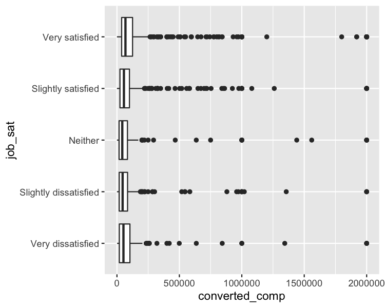
问题：不同工作满意度水平的年均薪酬是否不同？

stack_overflow %>% 
  ggplot(aes(x = job_sat, y = converted_comp)) +
  geom_boxplot() +
  coord_flip()

箱线图：5 个类别的薪酬分布。"Very satisfied" 似乎略高，但不易判断。

方差分析（ANOVA）

mdl_comp_vs_job_sat <- lm(converted_comp ~ job_sat, data = stack_overflow)

anova(mdl_comp_vs_job_sat)

Analysis of Variance Table

Response: converted_comp
            Df   Sum Sq  Mean Sq F value Pr(>F)   
job_sat      4 1.09e+12 2.73e+11    3.65 0.0057 **
Residuals 2570 1.92e+14 7.47e+10                  

Signif. codes:  0 '***' 0.001 '**' 0.01 '*' 0.05 '.' 0.1 ' ' 1

¹ "使用 lm() 的线性回归"见《R 回归入门》课程

两两检验

$\mu_{\text{very dissatisfied}} \neq \mu_{\text{slightly dissatisfied}}$
$\mu_{\text{very dissatisfied}} \neq \mu_{\text{neither}}$
$\mu_{\text{very dissatisfied}} \neq \mu_{\text{slightly satisfied}}$
$\mu_{\text{very dissatisfied}} \neq \mu_{\text{very satisfied}}$
$\mu_{\text{slightly dissatisfied}} \neq \mu_{\text{neither}}$

$\mu_{\text{slightly dissatisfied}} \neq \mu_{\text{slightly satisfied}}$
$\mu_{\text{slightly dissatisfied}} \neq \mu_{\text{very satisfied}}$
$\mu_{\text{neither}} \neq \mu_{\text{slightly satisfied}}$
$\mu_{\text{neither}} \neq \mu_{\text{very satisfied}}$
$\mu_{\text{slightly satisfied}} \neq \mu_{\text{very satisfied}}$

将显著性水平设为 $\alpha = 0.2$。

pairwise.t.test()

pairwise.t.test(stack_overflow$converted_comp, stack_overflow$job_sat, p.adjust.method = "none")

    Pairwise comparisons using t tests with pooled SD 

data:  stack_overflow$converted_comp and stack_overflow$job_sat 

                      Very dissatisfied Slightly dissatisfied Neither Slightly satisfied
Slightly dissatisfied 0.26860           -                     -       -                 
Neither               0.79578           0.36858               -       -                 
Slightly satisfied    0.29570           0.82931               0.41248 -                 
Very satisfied        0.34482           0.00384               0.15939 0.00084           

P value adjustment method: none

显著差异："Very satisfied" vs. "Slightly dissatisfied"；"Very satisfied" vs. "Neither"；"Very satisfied" vs. "Slightly satisfied"

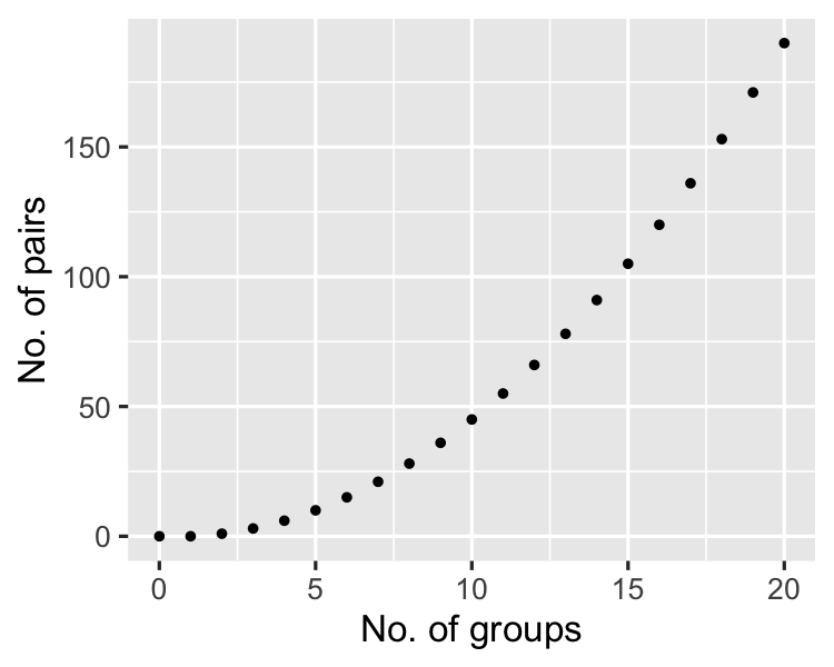
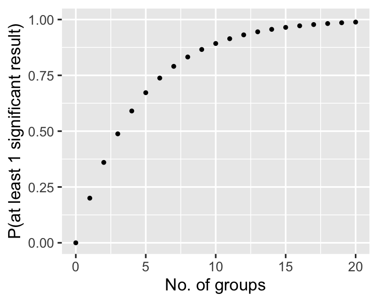
随着组数增加…

散点图：成对比较数量 vs. 组数。组数增加时，成对数量按二次关系增长。

散点图：至少得到1个显著结果的概率 vs. 组数。组数越多，至少1个显著结果的概率越高。

Bonferroni 校正

pairwise.t.test(stack_overflow$converted_comp, stack_overflow$job_sat, p.adjust.method = "bonferroni")

    Pairwise comparisons using t tests with pooled SD 

data:  stack_overflow$converted_comp and stack_overflow$job_sat 

                      Very dissatisfied Slightly dissatisfied Neither Slightly satisfied
Slightly dissatisfied 1.0000            -                     -       -                 
Neither               1.0000            1.0000                -       -                 
Slightly satisfied    1.0000            1.0000                1.0000  -                 
Very satisfied        1.0000            0.0384                1.0000  0.0084            

P value adjustment method: bonferroni

显著差异："Very satisfied" vs. "Slightly dissatisfied"；"Very satisfied" vs. "Slightly satisfied"

Bonferroni 与 Holm 调整

p_values

0.268603 0.795778 0.295702 0.344819 0.368580 0.829315 0.003840 0.412482 0.159389 0.000838

Bonferroni

pmin(1, 10 * p_values)

1.00000 1.00000 1.00000 1.00000 1.00000 1.00000 0.03840 1.00000 1.00000 0.00838

Holm（近似）

pmin(1, 10:1 * sort(p_values))

0.00838 0.03456 1.00000 1.00000 1.00000 1.00000 1.00000 1.00000 1.00000 0.82931

Passons à la pratique !