量化逻辑回归拟合

使用 Python 中的 statsmodels 进行回归入门

Maarten Van den Broeck

Content Developer at DataCamp

四种结果

	预测为假	预测为真
实际为假	正确	假阳性
实际为真	假阴性	正确

混淆矩阵：结果计数

actual_response = churn["has_churned"]

predicted_response = np.round(mdl_recency.predict())

outcomes = pd.DataFrame({"actual_response": actual_response,
                         "predicted_response": predicted_response})

print(outcomes.value_counts(sort=False))

actual_response  predicted_response
0                0.0                   141
                 1.0                    59
1                0.0                   111
                 1.0                    89

可视化混淆矩阵

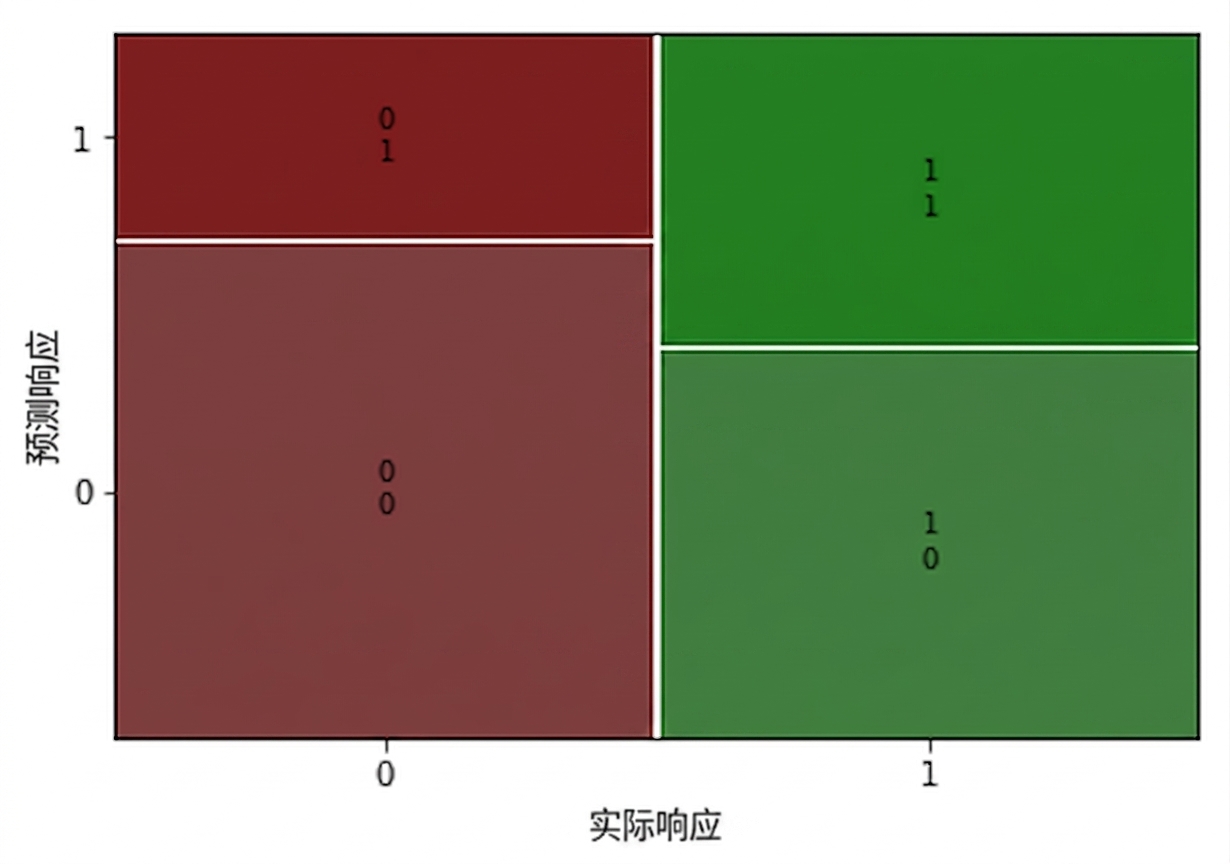
conf_matrix = mdl_recency.pred_table()

print(conf_matrix)

[[141.              59.]
 [111.              89.]]

真阴性	假阳性
假阴性	真阳性

from statsmodels.graphics.mosaicplot
import mosaic

mosaic(conf_matrix)

关于流失与最近一次活跃模型结果的马赛克图。真实流失和真实未流失各有 200 个观测，因此每列宽度相同。

准确率

"准确率"（Accuracy）是正确预测的比例。

$$ \text{accuracy} = \frac{TN + TP}{TN + FN + FP + TP} $$

 [[141.,  59.],
  [111.,  89.]]

TN = conf_matrix[0,0]
TP = conf_matrix[1,1]
FN = conf_matrix[1,0]
FP = conf_matrix[0,1]

acc = (TN + TP) / (TN + TP + FN + FP)
print(acc)

0.575

灵敏度

"灵敏度"（Sensitivity）是真阳性的比例。

$$ \text{sensitivity} = \frac{TP}{FN + TP} $$

 [[141.,  59.],
  [111.,  89.]]

TN = conf_matrix[0,0]
TP = conf_matrix[1,1]
FN = conf_matrix[1,0]
FP = conf_matrix[0,1]

sens = TP / (FN + TP)
print(sens)

0.445

特异度

"特异度"（Specificity）是真阴性的比例。

$$ \text{specificity} = \frac{TN}{TN + FP} $$

 [[141.,  59.],
  [111.,  89.]]

TN = conf_matrix[0,0]
TP = conf_matrix[1,1]
FN = conf_matrix[1,0]
FP = conf_matrix[0,1]

spec = TN / (TN + FP)
print(spec)

0.705

Vamos praticar!

使用 Python 中的 statsmodels 进行回归入门