使用 Python 中的 statsmodels 进行回归入门
Maarten Van den Broeck
Content Developer at DataCamp
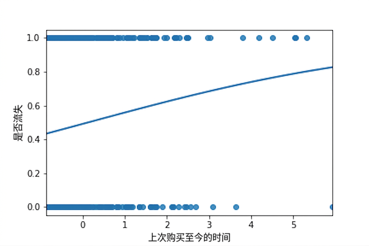
sns.regplot(x="time_since_last_purchase",
            y="has_churned",
            data=churn,
            ci=None,
            logistic=True)

plt.show()
mdl_recency = logit("has_churned ~ time_since_last_purchase",
                    data = churn).fit()


explanatory_data = pd.DataFrame(
  {"time_since_last_purchase": np.arange(-1, 6.25, 0.25)})


prediction_data = explanatory_data.assign(
    has_churned = mdl_recency.predict(explanatory_data))
mdl_recency = logit("has_churned ~ time_since_last_purchase", data = churn).fit()
explanatory_data = pd.DataFrame( {"time_since_last_purchase": np.arange(-1, 6.25, 0.25)})
prediction_data = explanatory_data.assign( has_churned = mdl_recency.predict(explanatory_data))
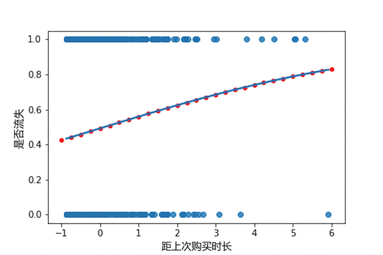
sns.regplot(x="time_since_last_purchase",
            y="has_churned",
            data=churn,
            ci=None,
            logistic=True)

sns.scatterplot(x="time_since_last_purchase",
                y="has_churned",
                data=prediction_data,
                color="red")

plt.show()
prediction_data = explanatory_data.assign(
    has_churned = mdl_recency.predict(explanatory_data))

prediction_data["most_likely_outcome"] = np.round(prediction_data["has_churned"])
prediction_data["most_likely_outcome"] = np.round(prediction_data["has_churned"])
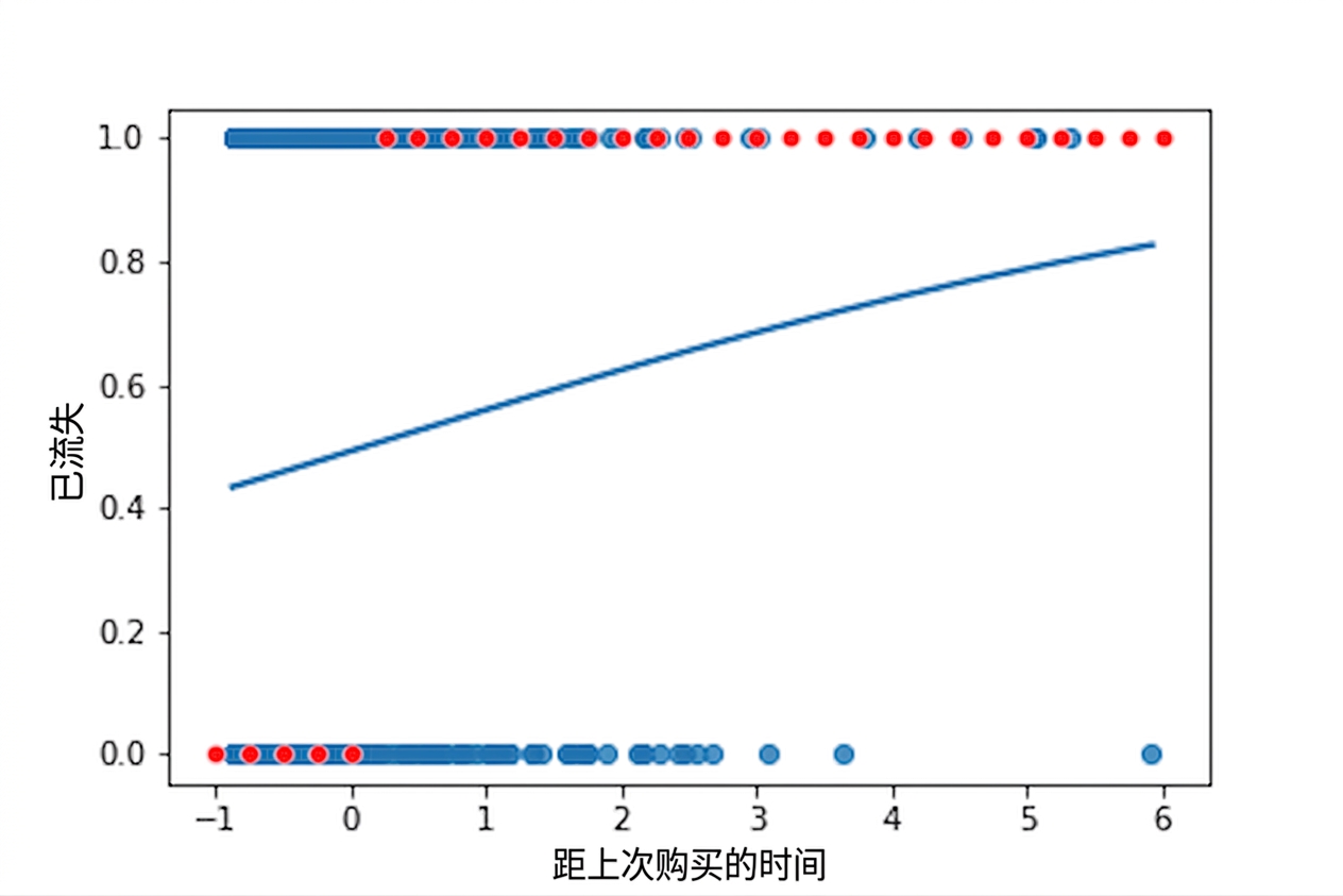
sns.regplot(x="time_since_last_purchase",
            y="has_churned",
            data=churn,
            ci=None,
            logistic=True)

sns.scatterplot(x="time_since_last_purchase",
                y="most_likely_outcome",
                data=prediction_data,
                color="red")

plt.show()
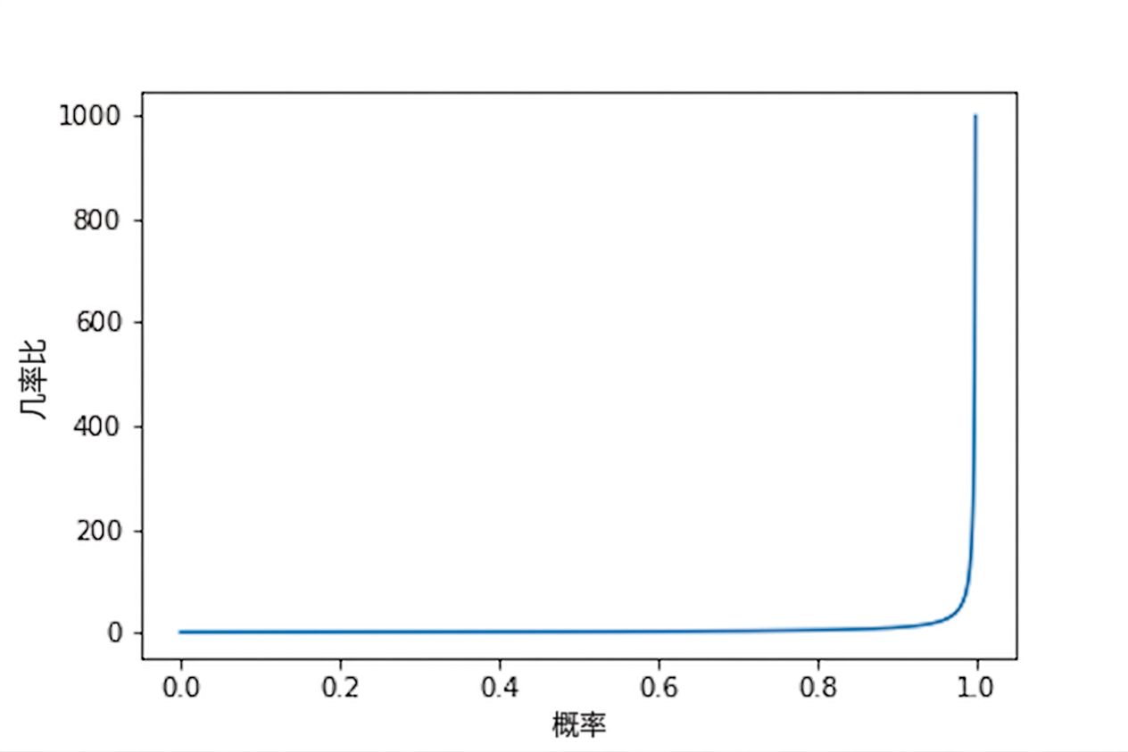
"赔率"是事件发生的概率除以其不发生的概率。
$$ \text{odds} = \frac{\text{probability}}{(1 - \text{probability)}} $$
$$ \text{odds} = \frac{0.25}{(1 - 0.25)} = \frac{1}{3} $$
prediction_data["odds"] = prediction_data["has_churned"] /
                            (1 - prediction_data["has_churned"])
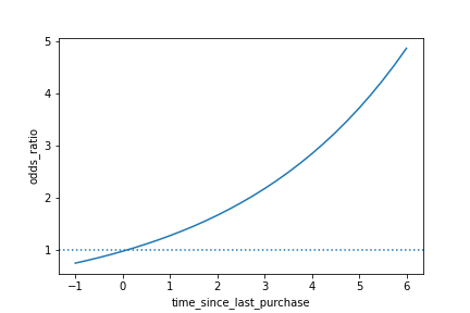
sns.lineplot(x="time_since_last_purchase",
             y="odds",
             data=prediction_data)


plt.axhline(y=1,
            linestyle="dotted")


plt.show()
sns.lineplot(x="time_since_last_purchase",
             y="odds",
             data=prediction_data)

plt.axhline(y=1,
            linestyle="dotted")
plt.show()
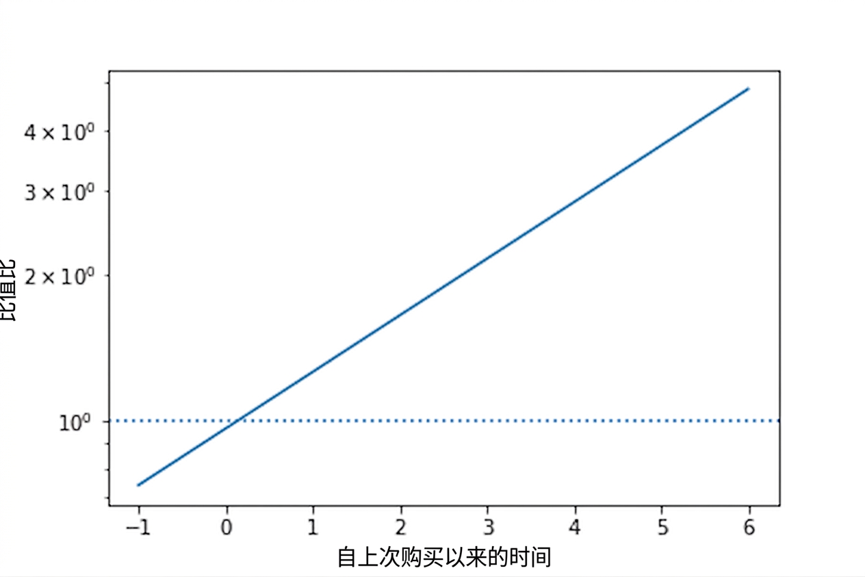
sns.lineplot(x="time_since_last_purchase", y="odds", data=prediction_data) plt.axhline(y=1, linestyle="dotted")
plt.yscale("log")

plt.show()
prediction_data["log_odds"] = np.log(prediction_data["odds"])