Diagrame de dispersie

Introducere în vizualizarea datelor cu ggplot2

Rick Scavetta

Founder, Scavetta Academy

48 de geometrii

geom_*
abline	contour	dotplot	jitter	pointrange	ribbon	spoke
area	count	errorbar	label	polygon	rug	step
bar	crossbar	errorbarh	line	qq	segment	text
bin2d	curve	freqpoly	linerange	qq_line	sf	tile
blank	density	hex	map	quantile	sf_label	violin
boxplot	density2d	histogram	path	raster	sf_text	vline
col	density_2d	hline	point	rect	smooth

Tipuri comune de grafice

Tip de grafic	Geomuri posibile
Diagrame de dispersie	points, jitter, abline, smooth, count

Diagrame de dispersie

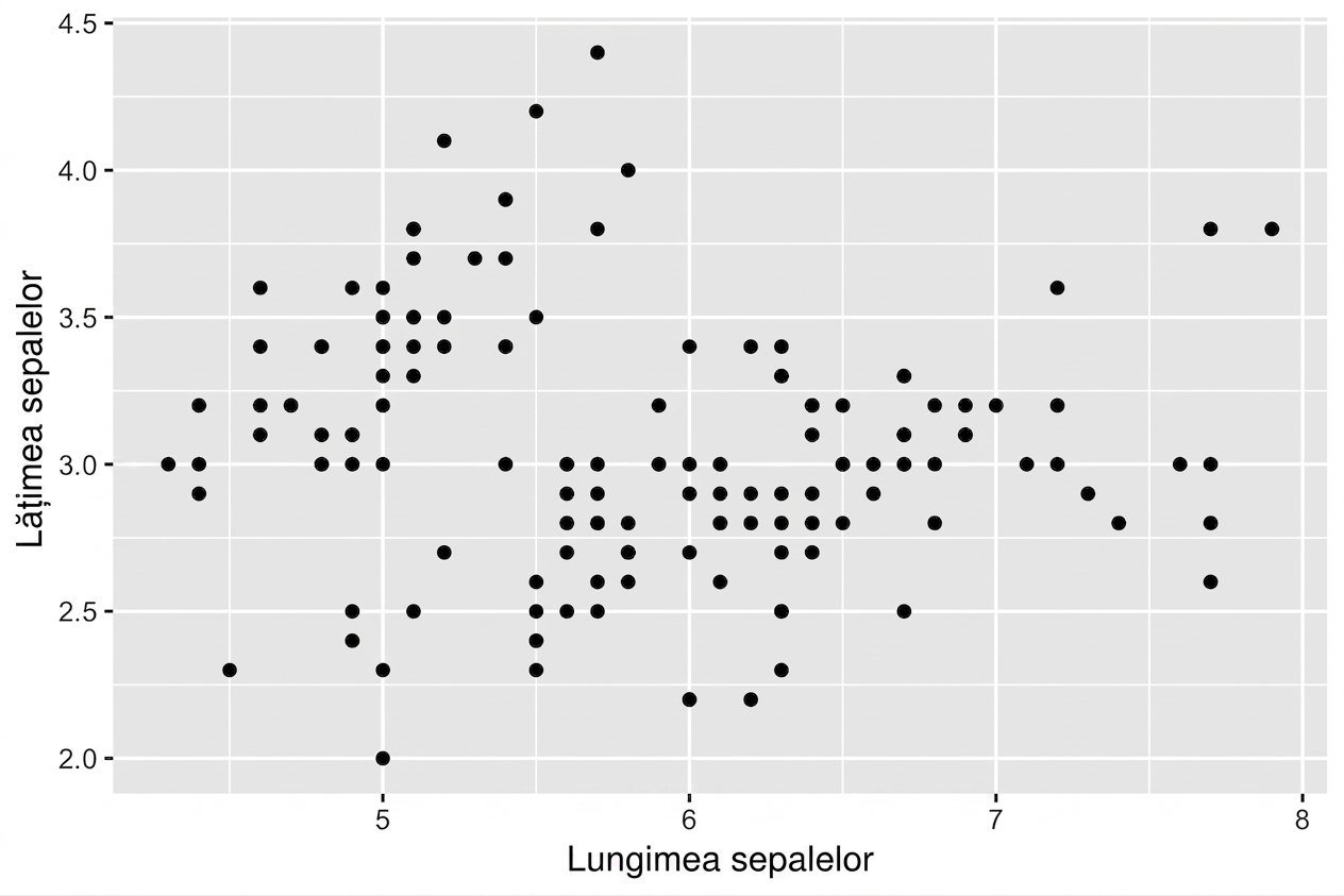
Fiecare geom acceptă mapări estetice specifice, de ex. geom_point():

Esențiale
x,y

ggplot(iris, aes(x = Sepal.Length, 
                 y = Sepal.Width)) + 
  geom_point()

Diagrame de dispersie

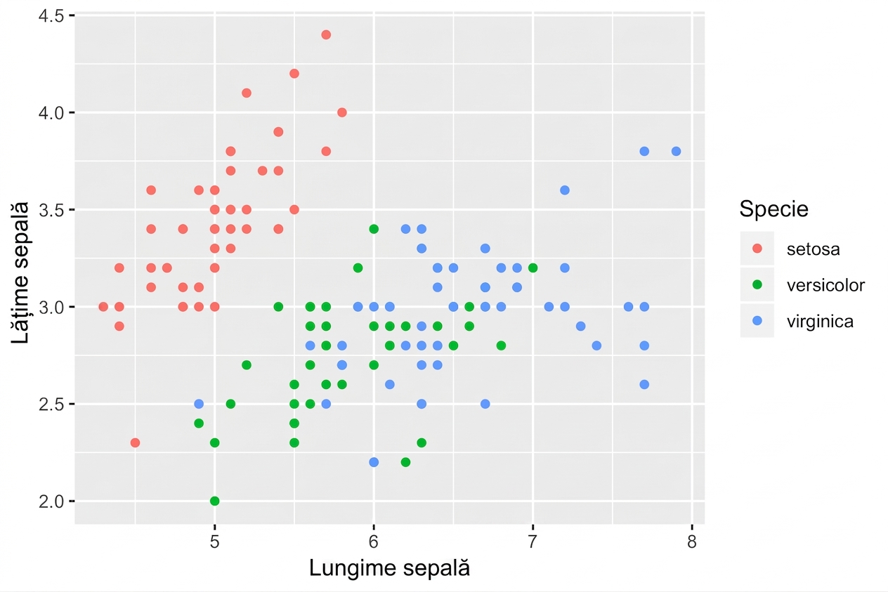
Fiecare geom acceptă mapări estetice specifice, de ex. geom_point():

Esențiale	Opționale
x,y	alpha, color, fill, shape, size, stroke

ggplot(iris, aes(x = Sepal.Length, 
                 y = Sepal.Width,
                 col = Species)) + 
  geom_point()

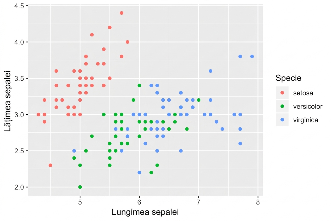
Mapări estetice specifice geomului

# These result in the same plot! 
ggplot(iris, aes(x = Sepal.Length, y = Sepal.Width, col = Species)) + 
  geom_point()

ggplot(iris, aes(x = Sepal.Length, y = Sepal.Width)) + 
  geom_point(aes(col = Species))

Controlați mapările estetice ale fiecărui strat independent:

head(iris, 3) # Raw data

Species Sepal.Length Sepal.Width Petal.Length Petal.Width
1  setosa          5.1         3.5          1.4         0.2
2  setosa          4.9         3.0          1.4         0.2
3  setosa          4.7         3.2          1.3         0.2

iris %>%
  group_by(Species) %>% 
  summarise_all(mean) -> iris.summary

iris.summary # Summary statistics

# A tibble: 3 x 5
  Species    Sepal.Length Sepal.Width Petal.Length Petal.Width
  <fct>             <dbl>       <dbl>        <dbl>       <dbl>
1 setosa             5.01        3.43         1.46       0.246
2 versicolor         5.94        2.77         4.26       1.33 
3 virginica          6.59        2.97         5.55       2.03

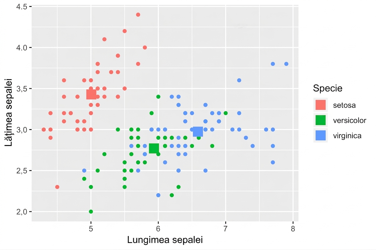
ggplot(iris, aes(x = Sepal.Length, y = Sepal.Width, col = Species)) +
  # Inherits both data and aes from ggplot() 
  geom_point() + 
  # Different data, but inherited aes
  geom_point(data = iris.summary, shape = 15, size = 5)

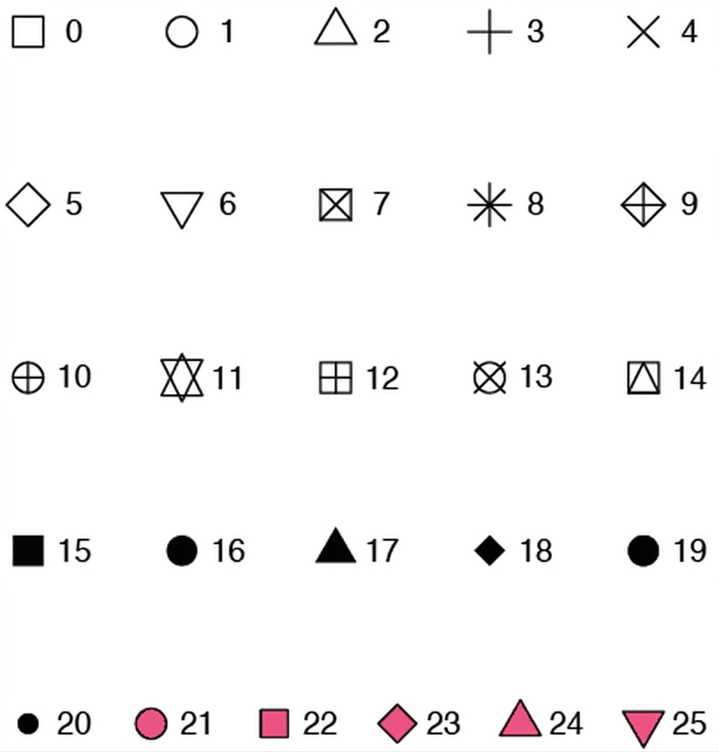
Valorile atributului shape

Exemplu

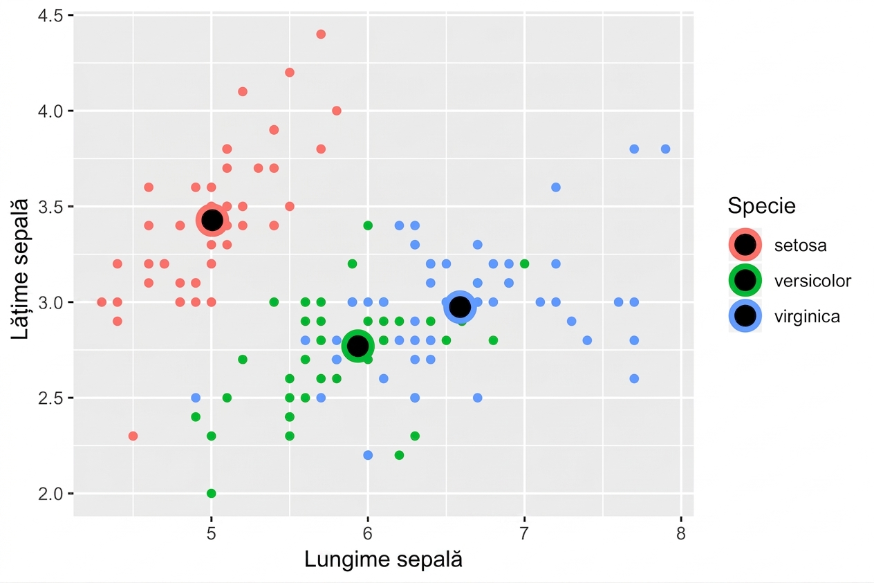
ggplot(iris, aes(x = Sepal.Length, y = Sepal.Width, col = Species)) + 
  geom_point() +
  geom_point(data = iris.summary, shape = 21, size = 5, 
             fill = "black", stroke = 2)

Statistici calculate din mers de ggplot2

Consultați cursul doi pentru stratul stats.
Notă: Evitați să reprezentați doar media fără o măsură a dispersiei, de ex. deviația standard.

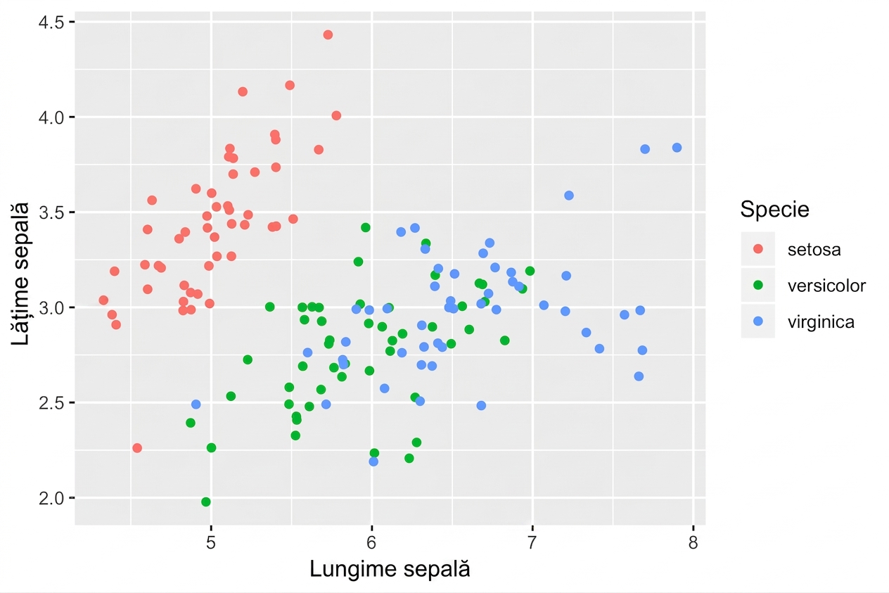
position = "jitter"

ggplot(iris, aes(x = Sepal.Length, y = Sepal.Width, col = Species)) + 
  geom_point(position = "jitter")

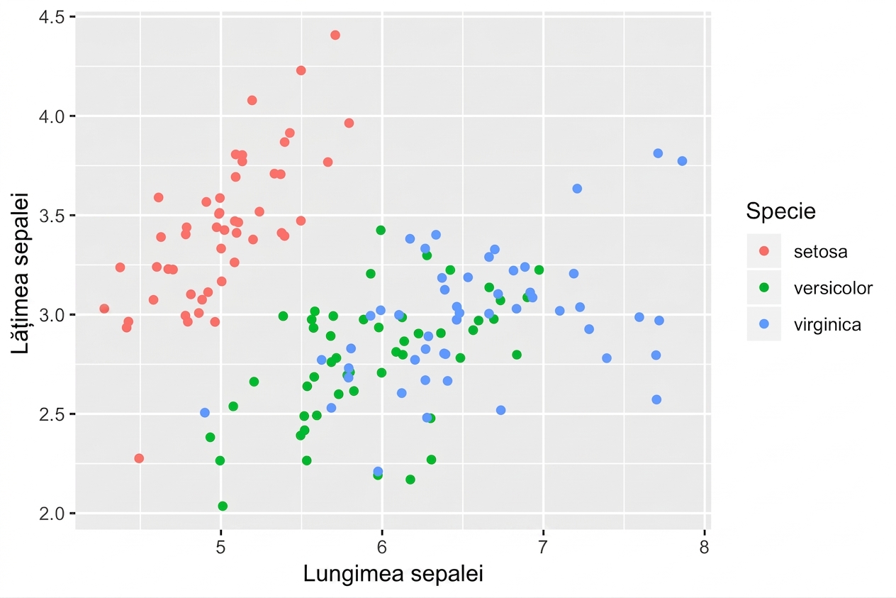
geom_jitter()

Prescurtare pentru geom_point(position = "jitter")

ggplot(iris, aes(x = Sepal.Length, y = Sepal.Width, col = Species)) + 
  geom_jitter()

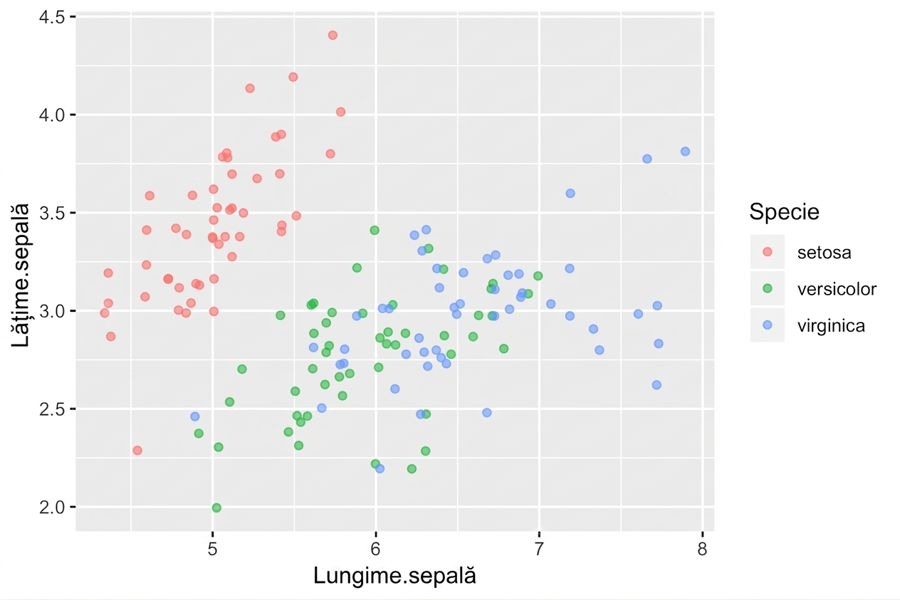
Nu uitați să ajustați alpha

Combinați jitteringul cu alpha-blending dacă este necesar

ggplot(iris, aes(x = Sepal.Length, y = Sepal.Width, col = Species)) + 
  geom_jitter(alpha = 0.6)

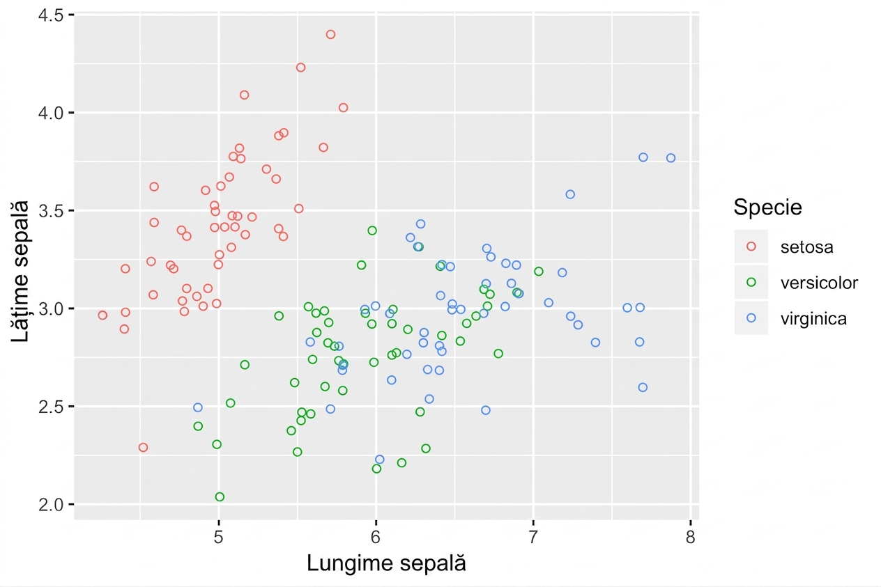
Cercurile goale ajută și ele

shape = 1 este un cerc gol.
Nu este necesară utilizarea suplimentară a alpha-blending.

ggplot(iris, aes(x = Sepal.Length, y = Sepal.Width, col = Species)) + 
  geom_jitter(shape = 1)

Să exersăm!

Introducere în vizualizarea datelor cu ggplot2