Introduction to Portfolio Risk Management in Python
Dakota Wixom
Quantitative Analyst | QuantCourse.com
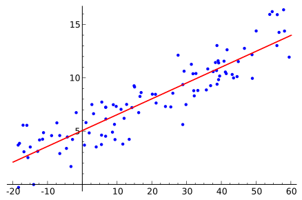
The Capital Asset Pricing Model is the fundamental building block for many other asset pricing models and factor models in finance.
To calculate excess returns, simply subtract the risk free rate of return from your total return:
$$ \text{Excess Return} = \text{Return} - \text{Risk Free Return} $$
Example:
Investing in Brazil:
10% Portfolio Return - 15% Risk Free Rate = -5% Excess Return
Investing in the US:
10% Portfolio Return - 3% Risk Free Rate = 7% Excess Return
$$ E(R_{P}) - RF = \beta_{{P}}(E(R_{M})-RF)\ $$
To calculate historical beta using co-variance:
$$ \beta_P = \frac{Cov(R_P, R_B)}{Var(R_B)} $$
Assuming you already have excess portfolio and market returns in the object Data
:
covariance_matrix = Data[["Port_Excess","Mkt_Excess"]].cov()
covariance_coefficient = covariance_matrix.iloc[0, 1]
benchmark_variance = Data["Mkt_Excess"].var()
portfolio_beta = covariance_coefficient / benchmark_variance
portfolio_beta
0.93
Example of a linear regression:
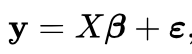
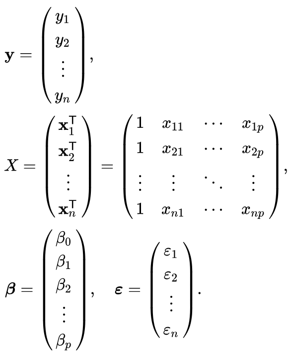
Regression formula in matrix notation:
Assuming you already have excess portfolio and market returns in the object Data
:
import statsmodels.formula.api as smf
model = smf.ols(formula='Port_Excess ~ Mkt_Excess', data=Data)
fit = model.fit()
beta = fit.params["Mkt_Excess"]
beta
0.93
To extract the adjusted r-squared and r-squared values:
import statsmodels.formula.api as smf
model = smf.ols(formula='Port_Excess ~ Mkt_Excess', data=Data)
fit = model.fit()
r_squared = fit.rsquared
r_squared
0.70
adjusted_r_squared = fit.rsquared_adj
0.65
Introduction to Portfolio Risk Management in Python