स्कैटर प्लॉट्स

ggplot2 के साथ डेटा विज़ुअलाइज़ेशन परिचय

Rick Scavetta

Founder, Scavetta Academy

48 ज्योमेट्रीज़

geom_*
abline	contour	dotplot	jitter	pointrange	ribbon	spoke
area	count	errorbar	label	polygon	rug	step
bar	crossbar	errorbarh	line	qq	segment	text
bin2d	curve	freqpoly	linerange	qq_line	sf	tile
blank	density	hex	map	quantile	sf_label	violin
boxplot	density2d	histogram	path	raster	sf_text	vline
col	density_2d	hline	point	rect	smooth

सामान्य प्लॉट प्रकार

प्लॉट प्रकार	संभावित Geoms
स्कैटर प्लॉट्स	points, jitter, abline, smooth, count

स्कैटर प्लॉट्स

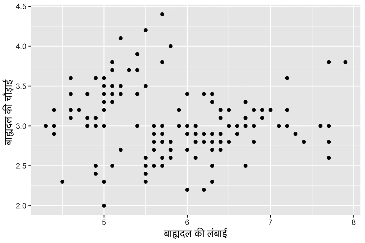
हर geom कुछ खास aesthetic mappings लेता है, जैसे geom_point():

आवश्यक
x,y

ggplot(iris, aes(x = Sepal.Length, 
                 y = Sepal.Width)) + 
  geom_point()

स्कैटर प्लॉट्स

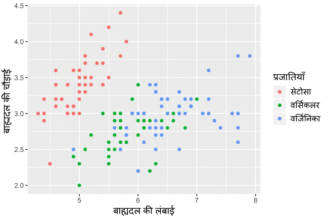
हर geom कुछ खास aesthetic mappings लेता है, जैसे geom_point():

Essential	Optional
x,y	alpha, color, fill, shape, size, stroke

ggplot(iris, aes(x = Sepal.Length, 
                 y = Sepal.Width,
                 col = Species)) + 
  geom_point()

Geom-विशिष्ट aesthetic mappings

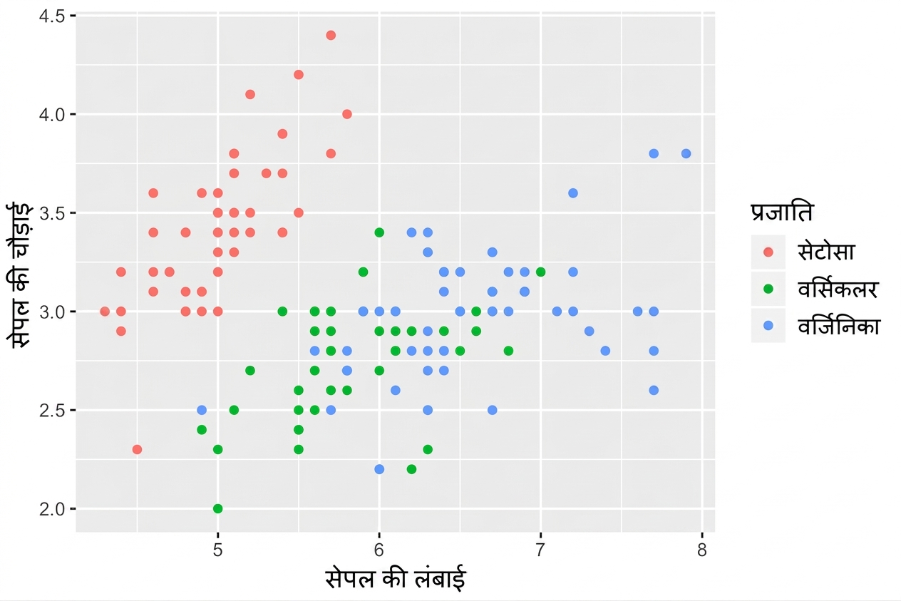
# ये दोनों एक जैसा प्लॉट देते हैं! 
ggplot(iris, aes(x = Sepal.Length, y = Sepal.Width, col = Species)) + 
  geom_point()

ggplot(iris, aes(x = Sepal.Length, y = Sepal.Width)) + 
  geom_point(aes(col = Species))

हर लेयर के aesthetic mappings अलग-अलग नियंत्रित करें:

head(iris, 3) # कच्चा डेटा

Species Sepal.Length Sepal.Width Petal.Length Petal.Width
1  setosa          5.1         3.5          1.4         0.2
2  setosa          4.9         3.0          1.4         0.2
3  setosa          4.7         3.2          1.3         0.2

iris %>%
  group_by(Species) %>% 
  summarise_all(mean) -> iris.summary

iris.summary # सार आँकड़े

# A tibble: 3 x 5
  Species    Sepal.Length Sepal.Width Petal.Length Petal.Width
  <fct>             <dbl>       <dbl>        <dbl>       <dbl>
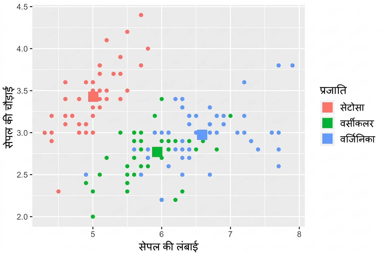
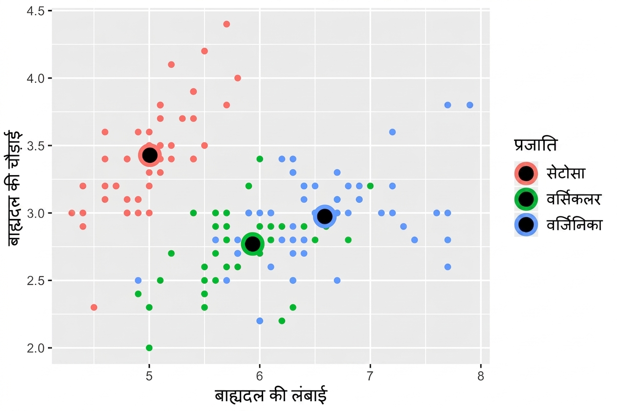
1 setosa             5.01        3.43         1.46       0.246
2 versicolor         5.94        2.77         4.26       1.33 
3 virginica          6.59        2.97         5.55       2.03

ggplot(iris, aes(x = Sepal.Length, y = Sepal.Width, col = Species)) +
  # ggplot() से data और aes दोनों इनहेरिट होते हैं 
  geom_point() + 
  # अलग data, लेकिन aes इनहेरिट
  geom_point(data = iris.summary, shape = 15, size = 5)

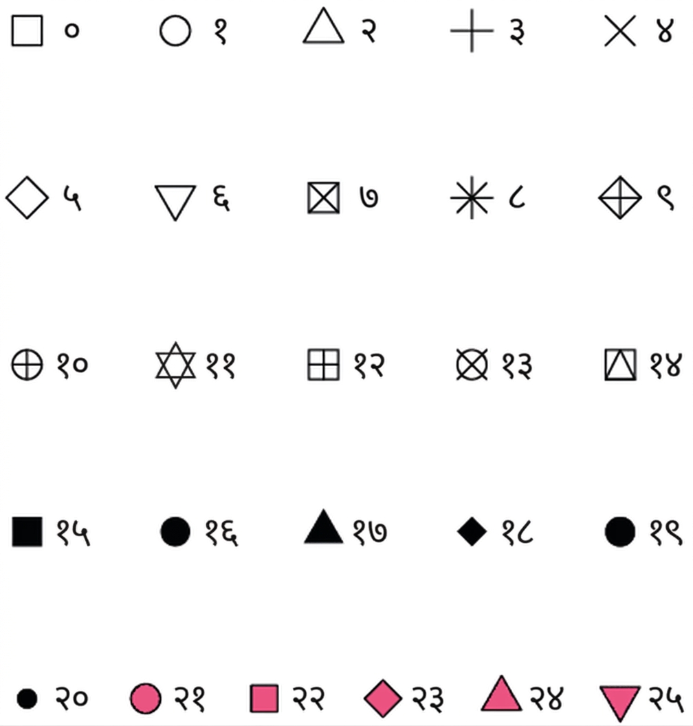
Shape एट्रीब्यूट मान

उदाहरण

ggplot(iris, aes(x = Sepal.Length, y = Sepal.Width, col = Species)) + 
  geom_point() +
  geom_point(data = iris.summary, shape = 21, size = 5, 
             fill = "black", stroke = 2)

ggplot2 द्वारा ऑन-द-फ्लाई stats

stats लेयर के लिए दूसरा कोर्स देखें.
ध्यान दें: केवल mean को बिना फैलाव के माप के न प्लॉट करें, जैसे standard deviation.

position = "jitter"

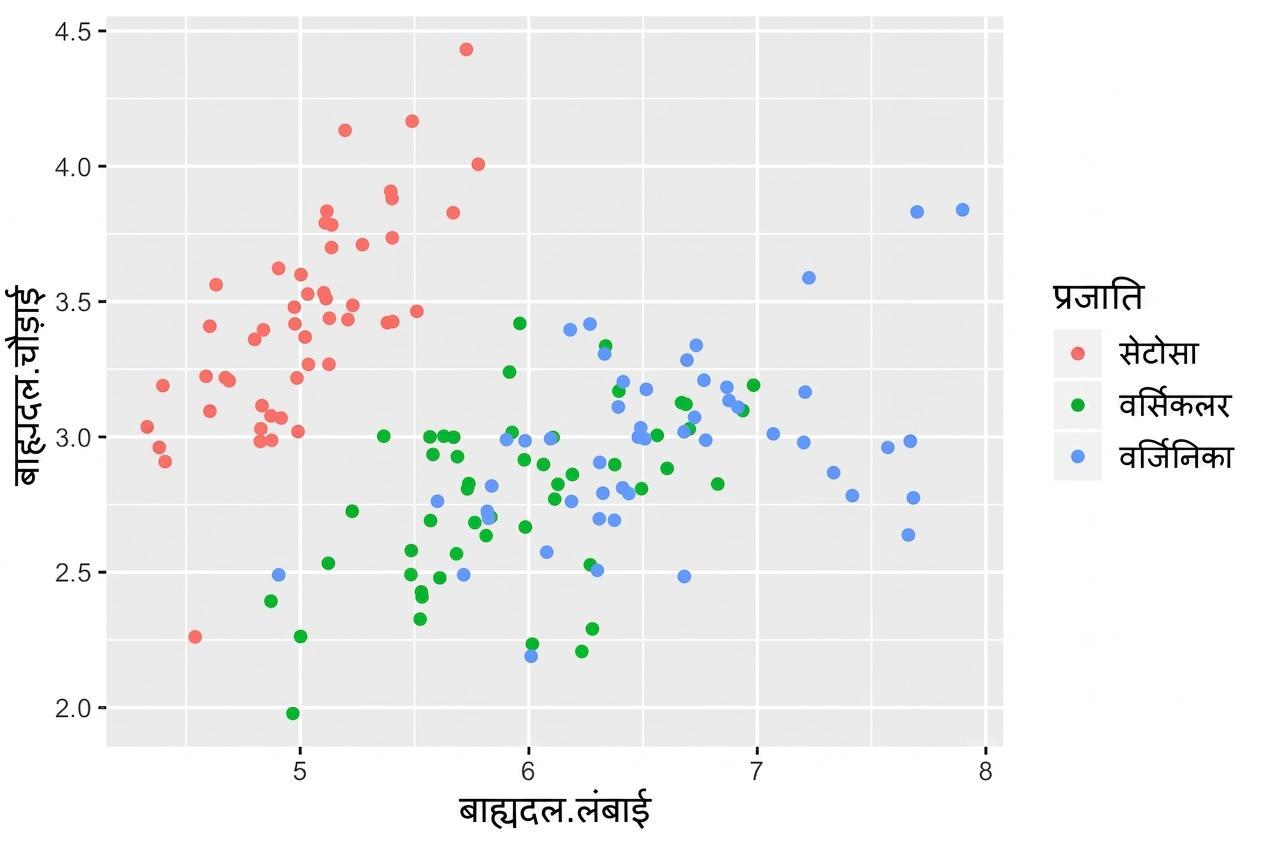
ggplot(iris, aes(x = Sepal.Length, y = Sepal.Width, col = Species)) + 
  geom_point(position = "jitter")

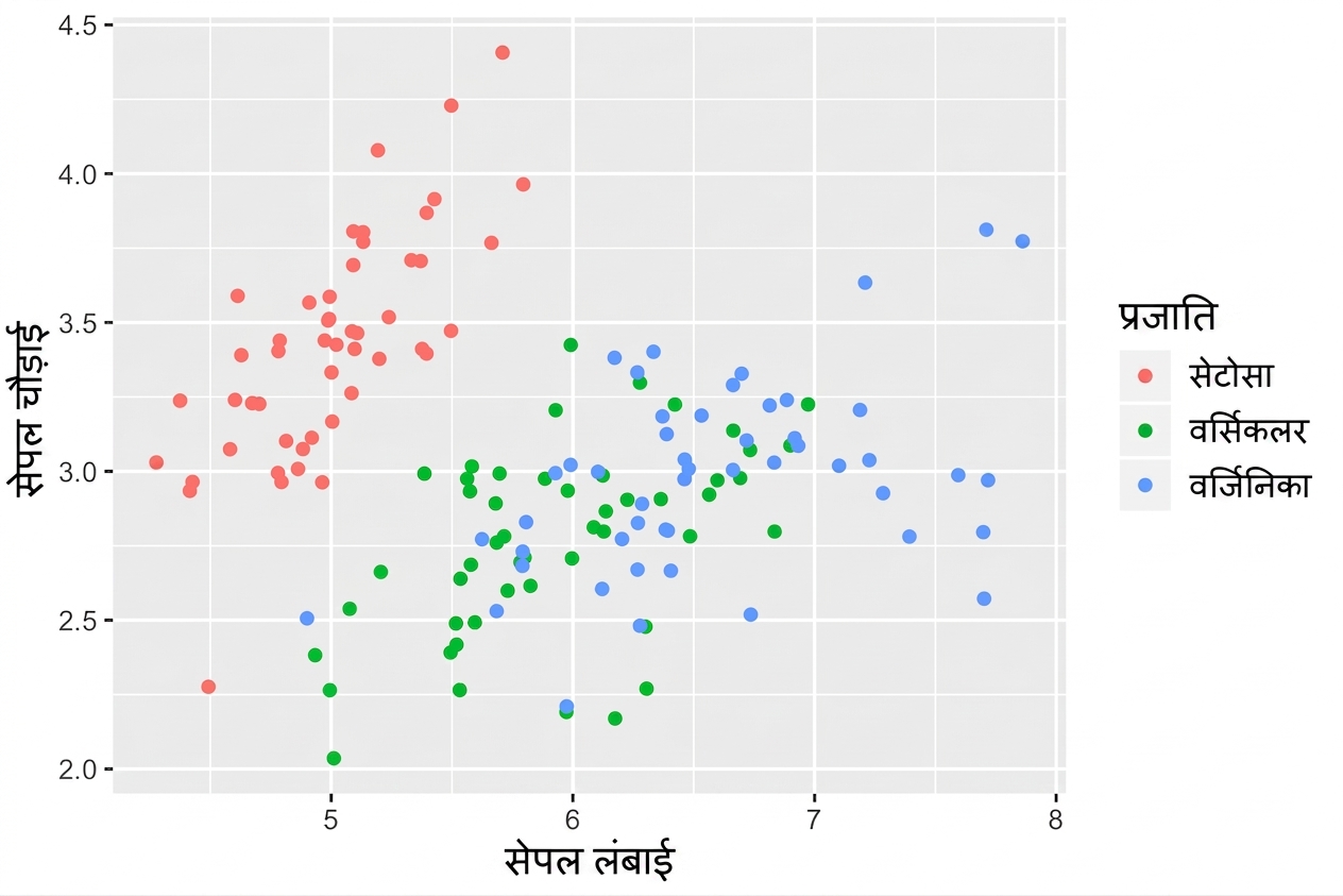
geom_jitter()

geom_point(position = "jitter") का शॉर्टकट

ggplot(iris, aes(x = Sepal.Length, y = Sepal.Width, col = Species)) + 
  geom_jitter()

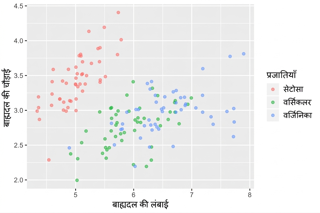
alpha समायोजित करना न भूलें

ज़रूरत हो तो jittering को alpha-blending के साथ मिलाएँ

ggplot(iris, aes(x = Sepal.Length, y = Sepal.Width, col = Species)) + 
  geom_jitter(alpha = 0.6)

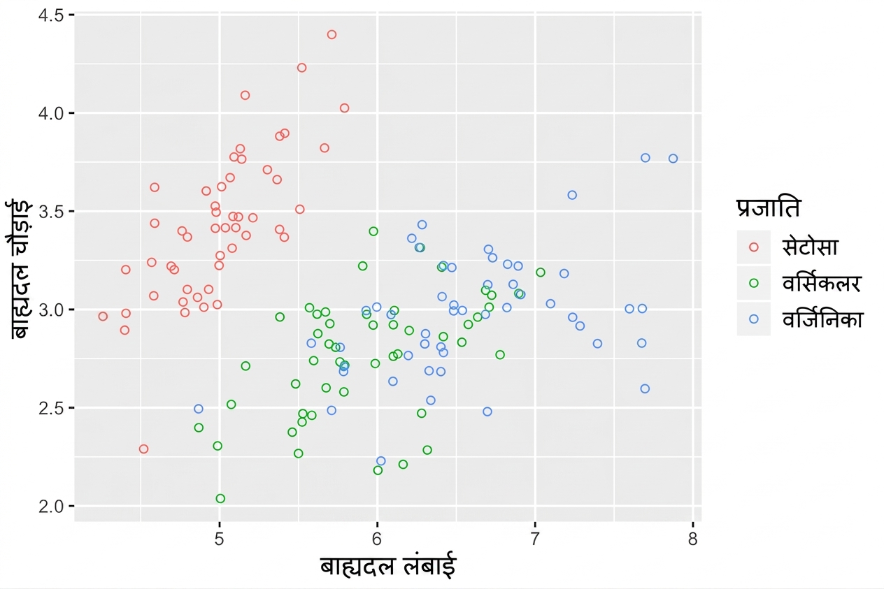
होलो सर्कल भी मदद करते हैं

shape = 1 एक खोखला सर्कल है.
तब alpha-blending की ज़रूरत नहीं रहती.

ggplot(iris, aes(x = Sepal.Length, y = Sepal.Width, col = Species)) + 
  geom_jitter(shape = 1)

अभ्यास करते हैं!

ggplot2 के साथ डेटा विज़ुअलाइज़ेशन परिचय