Scatter plots

การแสดงผลข้อมูลด้วย ggplot2 เบื้องต้น

Rick Scavetta

Founder, Scavetta Academy

48 geometries

geom_*
abline	contour	dotplot	jitter	pointrange	ribbon	spoke
area	count	errorbar	label	polygon	rug	step
bar	crossbar	errorbarh	line	qq	segment	text
bin2d	curve	freqpoly	linerange	qq_line	sf	tile
blank	density	hex	map	quantile	sf_label	violin
boxplot	density2d	histogram	path	raster	sf_text	vline
col	density_2d	hline	point	rect	smooth

ประเภทพล็อตที่พบบ่อย

ประเภทพล็อต	Geoms ที่ใช้ได้
Scatter plots	points, jitter, abline, smooth, count

Scatter plots

แต่ละ geom รับ aesthetic mapping เฉพาะของตัวเอง เช่น geom_point():

จำเป็น
x,y

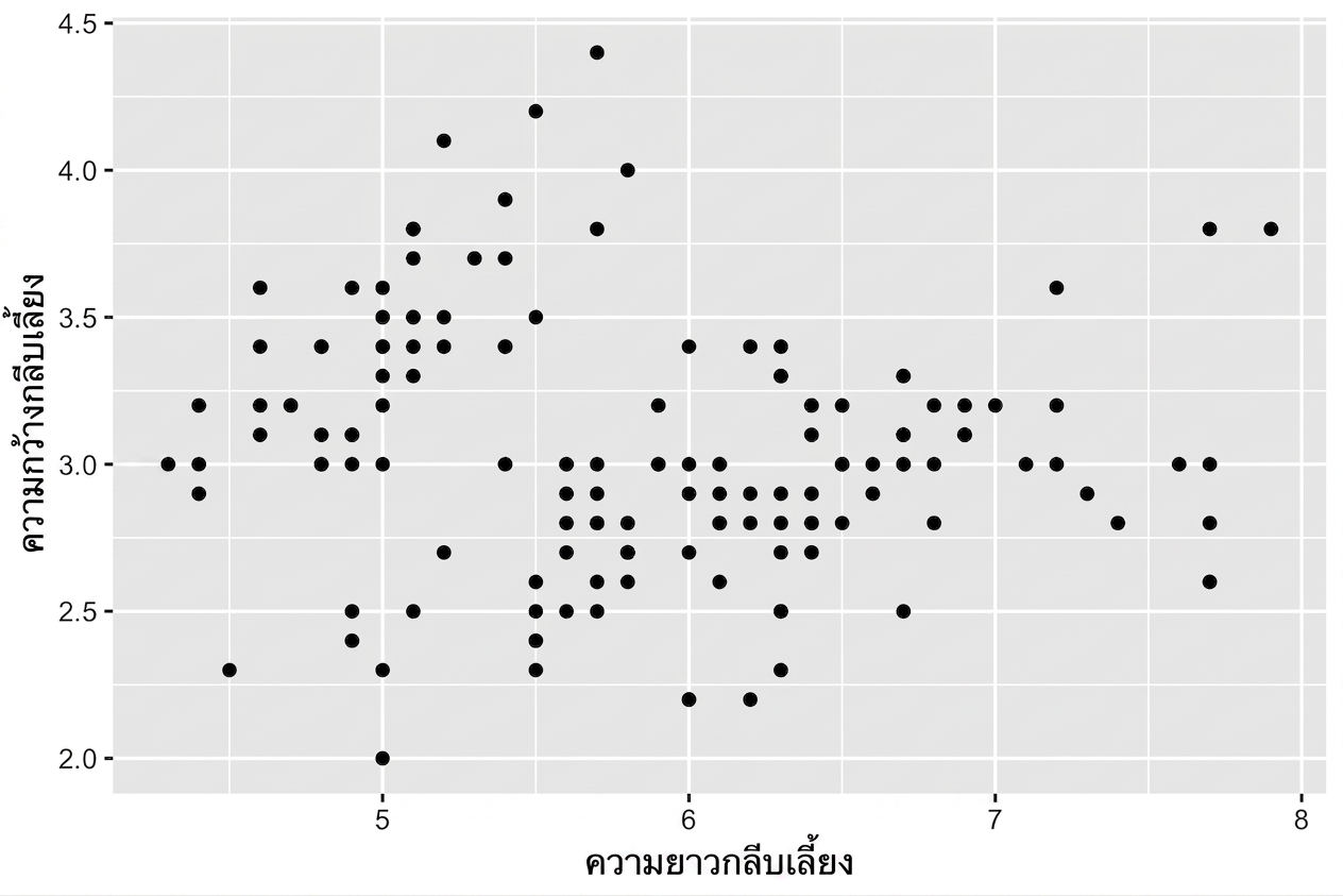
ggplot(iris, aes(x = Sepal.Length, 
                 y = Sepal.Width)) + 
  geom_point()

Scatter plots

แต่ละ geom รับ aesthetic mapping เฉพาะของตัวเอง เช่น geom_point():

จำเป็น	ไม่บังคับ
x,y	alpha, color, fill, shape, size, stroke

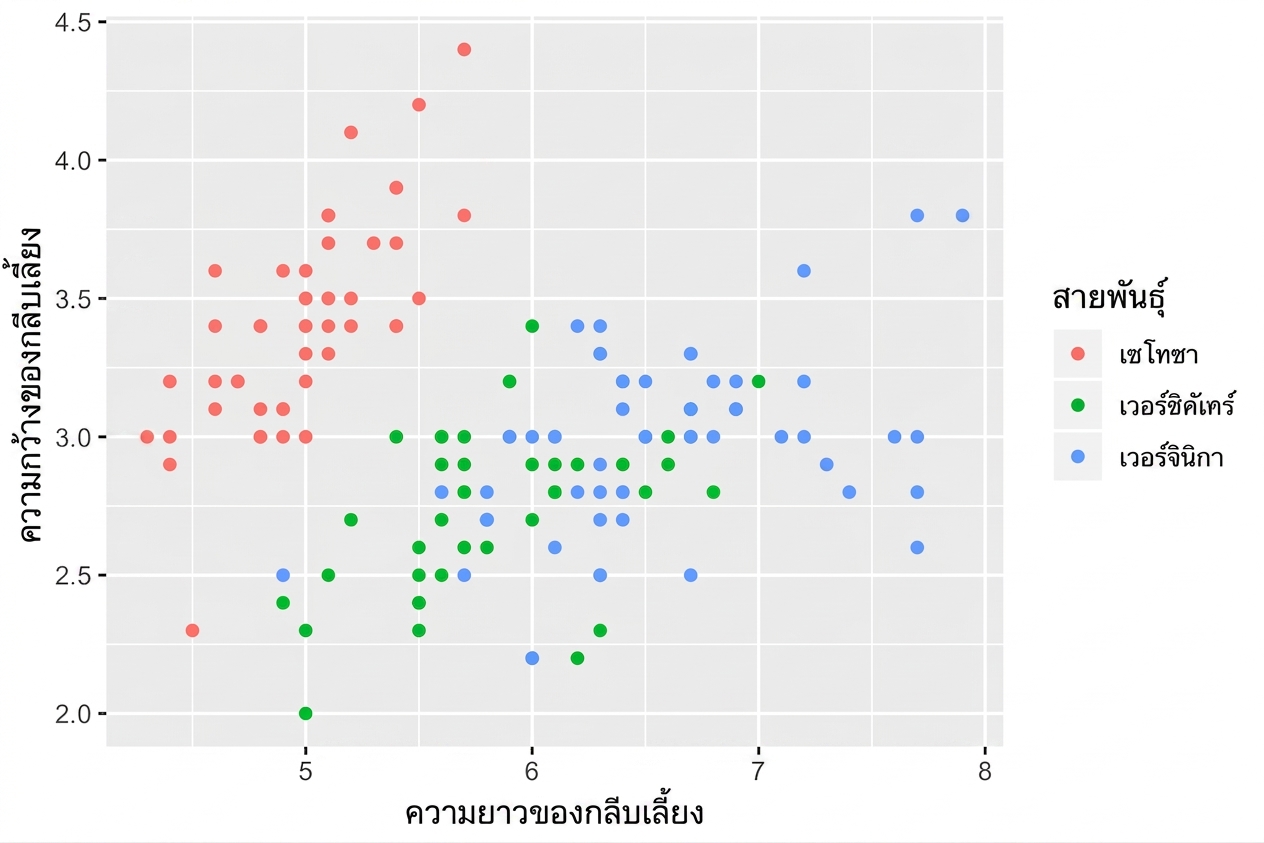
ggplot(iris, aes(x = Sepal.Length, 
                 y = Sepal.Width,
                 col = Species)) + 
  geom_point()

Aesthetic mapping เฉพาะของแต่ละ geom

# These result in the same plot! 
ggplot(iris, aes(x = Sepal.Length, y = Sepal.Width, col = Species)) + 
  geom_point()

ggplot(iris, aes(x = Sepal.Length, y = Sepal.Width)) + 
  geom_point(aes(col = Species))

ควบคุม aesthetic mapping ของแต่ละ layer อย่างอิสระ:

head(iris, 3) # Raw data

Species Sepal.Length Sepal.Width Petal.Length Petal.Width
1  setosa          5.1         3.5          1.4         0.2
2  setosa          4.9         3.0          1.4         0.2
3  setosa          4.7         3.2          1.3         0.2

iris %>%
  group_by(Species) %>% 
  summarise_all(mean) -> iris.summary

iris.summary # Summary statistics

# A tibble: 3 x 5
  Species    Sepal.Length Sepal.Width Petal.Length Petal.Width
  <fct>             <dbl>       <dbl>        <dbl>       <dbl>
1 setosa             5.01        3.43         1.46       0.246
2 versicolor         5.94        2.77         4.26       1.33 
3 virginica          6.59        2.97         5.55       2.03

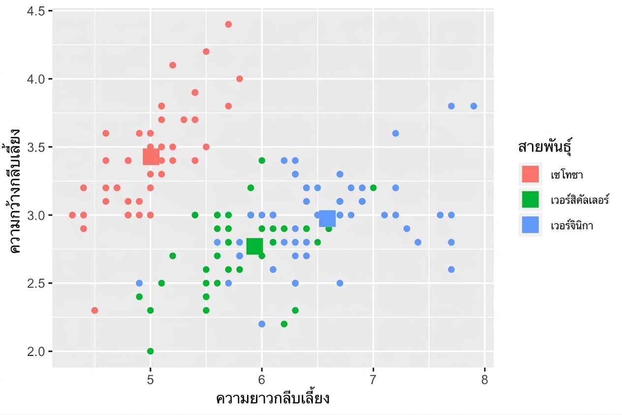
ggplot(iris, aes(x = Sepal.Length, y = Sepal.Width, col = Species)) +
  # Inherits both data and aes from ggplot() 
  geom_point() + 
  # Different data, but inherited aes
  geom_point(data = iris.summary, shape = 15, size = 5)

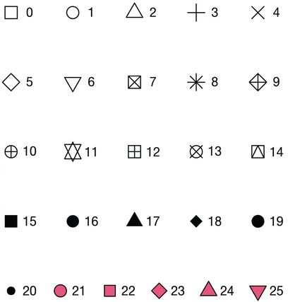
ค่าของแอตทริบิวต์ shape

ตัวอย่าง

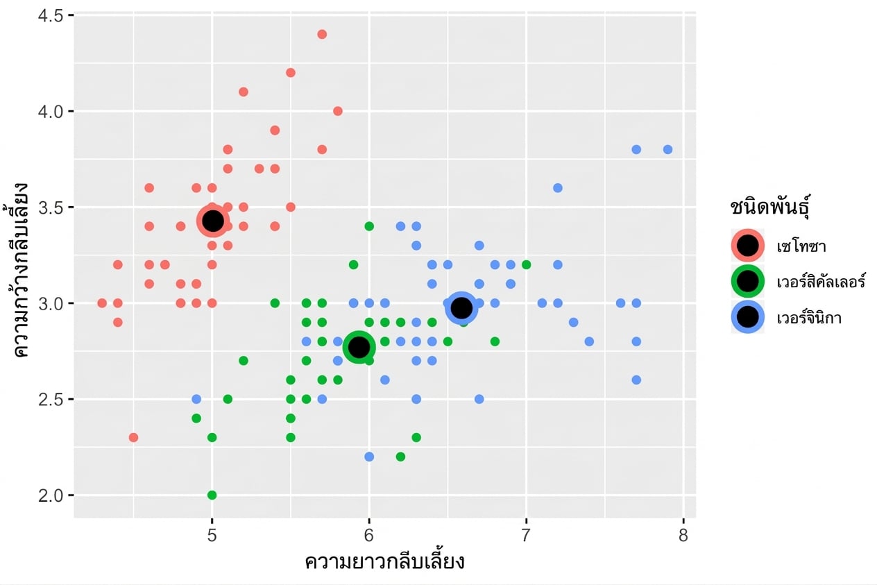
ggplot(iris, aes(x = Sepal.Length, y = Sepal.Width, col = Species)) + 
  geom_point() +
  geom_point(data = iris.summary, shape = 21, size = 5, 
             fill = "black", stroke = 2)

การคำนวณสถิติอัตโนมัติโดย ggplot2

ดู stats layer ได้ในคอร์สที่สอง
หมายเหตุ: หลีกเลี่ยงการพล็อตเฉพาะค่าเฉลี่ยโดยไม่แสดงการกระจาย เช่น ส่วนเบี่ยงเบนมาตรฐาน

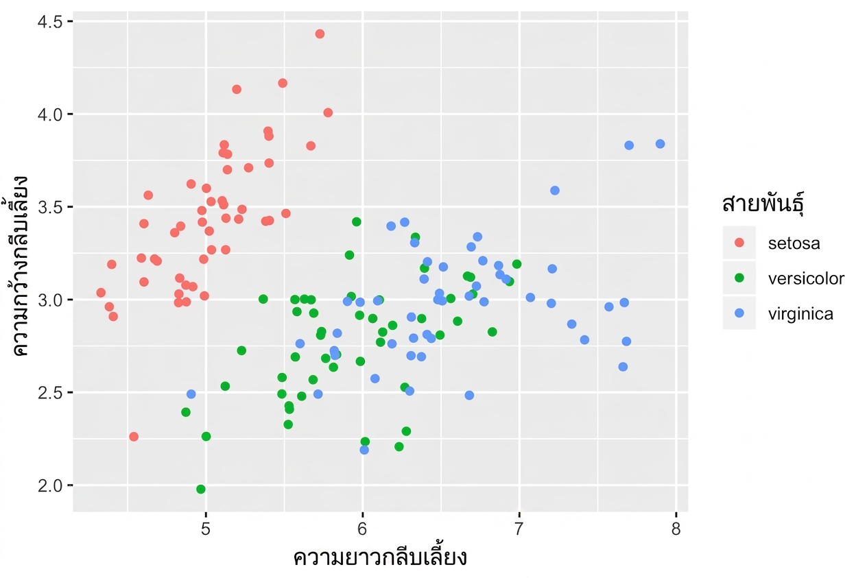
position = "jitter"

ggplot(iris, aes(x = Sepal.Length, y = Sepal.Width, col = Species)) + 
  geom_point(position = "jitter")

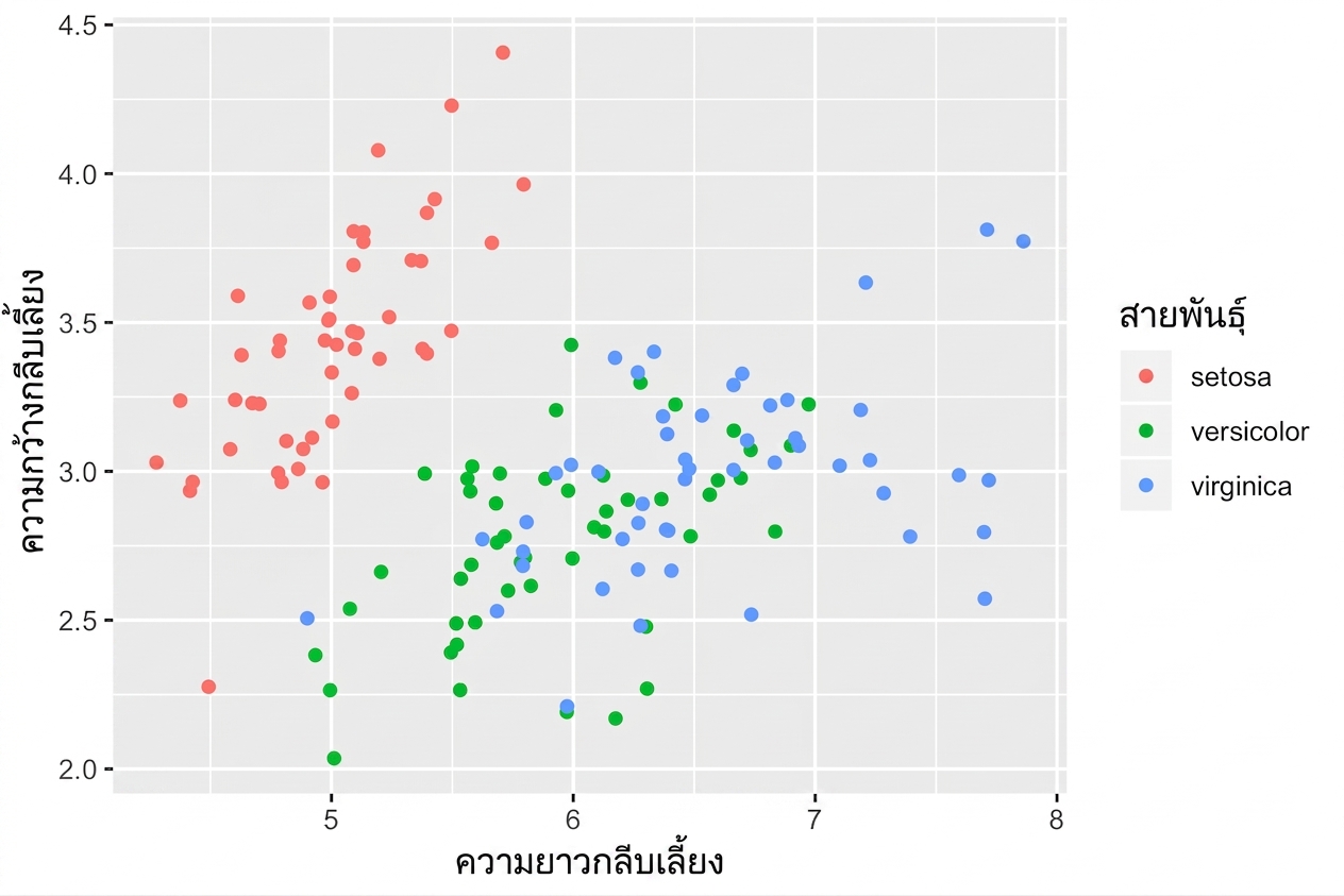
geom_jitter()

รูปแบบย่อของ geom_point(position = "jitter")

ggplot(iris, aes(x = Sepal.Length, y = Sepal.Width, col = Species)) + 
  geom_jitter()

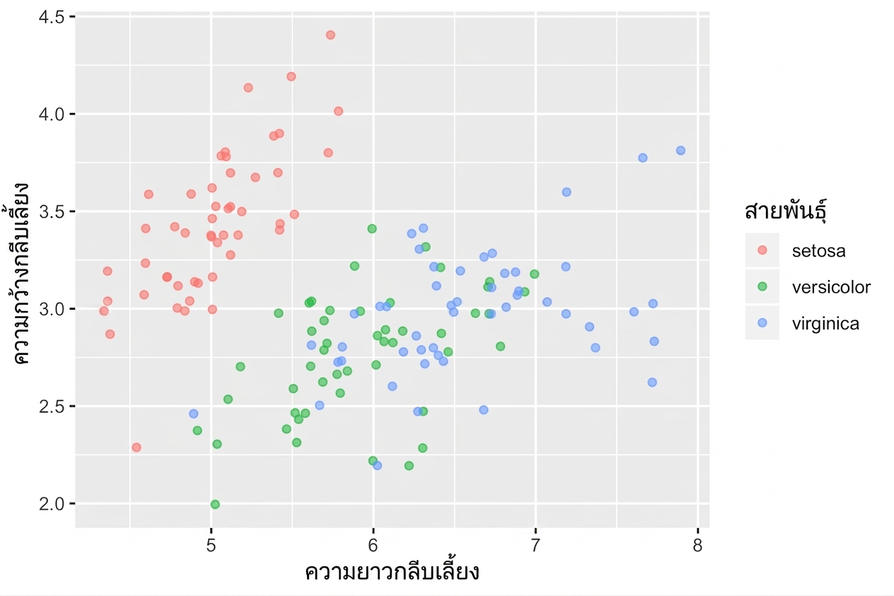
อย่าลืมปรับค่า alpha

ใช้ jittering ร่วมกับ alpha-blending เมื่อจำเป็น

ggplot(iris, aes(x = Sepal.Length, y = Sepal.Width, col = Species)) + 
  geom_jitter(alpha = 0.6)

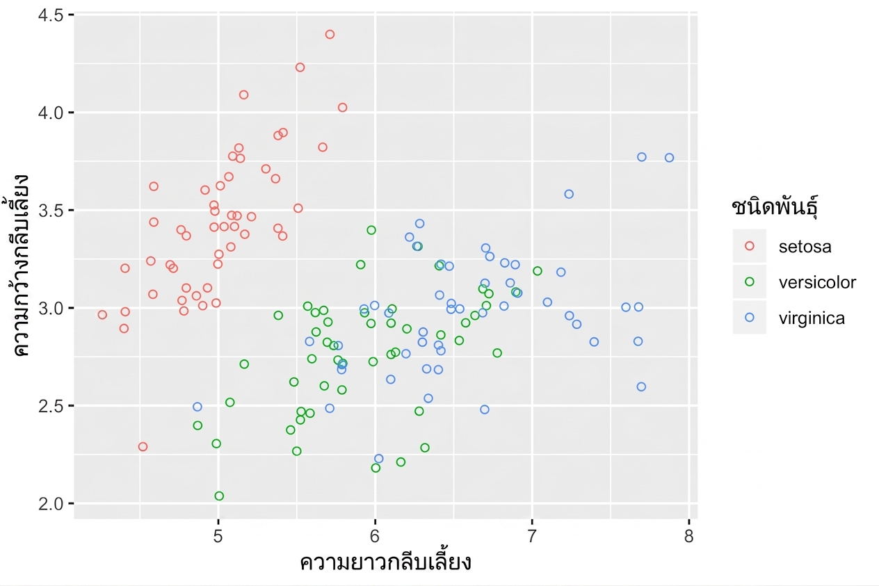
วงกลมกลวงช่วยได้เช่นกัน

shape = 1 คือวงกลมกลวง
ไม่จำเป็นต้องใช้ alpha-blending ร่วมด้วย

ggplot(iris, aes(x = Sepal.Length, y = Sepal.Width, col = Species)) + 
  geom_jitter(shape = 1)

มาฝึกกันเถอะ!

การแสดงผลข้อมูลด้วย ggplot2 เบื้องต้น